There are several ways to solvrow transformation method, inverse matrix method and so on. The triangular decomposition method is also one of that.e a set of equations in matrix algebra like Gaussian elimination method,
Here I’ll only work with the 3 × 3 matrices. Soon, I’ll also write on the triangular decomposition method in 4 × 4 matrices.
Here I’ll explain how to use the row transformation method to solve a set of equations.
METHOD
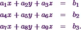
Suppose I have a set of equations like
Now I have to solve these equations using the triangular decomposition method.
Step 1
First of all, I’ll write the set of equations in a matrix form.
Thus it will be
![\[ \begin{pmatrix} a_1&a_2&a_3\\ a_4 &a_5 &a_6\\ a_7 &a_8 &a_9 \end{pmatrix}\begin{pmatrix} x\\ y\\ z \end{pmatrix}=\begin{pmatrix} b_1\\ b_2\\ b_3 \end{pmatrix}. \]](https://appassets.softecksblog.in/engineering_mathematics/assets/em2/12_files/image002.webp)
So I can say the system of equations is in the form of  .
.
Here  is the coefficient matrix,
  is the variable matrix and
  is the constant matrix.
In the method of triangular decomposition, the first task is to write the coefficient matrix as a product of two matrices  and
and  .
.
The matrix will be a lower triangular matrix. And, the matrix will be an upper triangular matrix.
Thus it will be  .
.
Here the matrix will look like
![\[ \textbf{L} = \begin{pmatrix} l_{11}&0&0\\ l_{21} &l_{22} &0\\ l_{31} &l_{32} &l_{33} \end{pmatrix}. \]](https://appassets.softecksblog.in/engineering_mathematics/assets/em2/12_files/image010.webp)
Similarly, the matrix will be
![\[ \textbf{U} = \begin{pmatrix} 1&u_{12}&u_{13}\\ 0 &1 &u_{23}\\ 0 &0 &1 \end{pmatrix}. \]](https://appassets.softecksblog.in/engineering_mathematics/assets/em2/12_files/image011.webp)
Thus the system of equations will be
![\[\textbf{A x = b} \Rightarrow \textbf{(L U) x = b}.\]](https://appassets.softecksblog.in/engineering_mathematics/assets/em2/12_files/image012.webp)
Step 2
Now I’ll choose  .
.
Here the matrix  will be
![\[ \textbf{y} = \begin{pmatrix} y_1\\ y_2\\ y_3 \end{pmatrix}. \]](https://appassets.softecksblog.in/engineering_mathematics/assets/em2/12_files/image015.webp)
So I can say
![\[\textbf{A x = b} \Rightarrow \textbf{L (U x) = b} \Rightarrow \textbf{L y= b}.\]](https://appassets.softecksblog.in/engineering_mathematics/assets/em2/12_files/image016.webp)
Then I’ll solve for . Next, I’ll solve for using the relation .
Now I’ll solve an example on that.
EXAMPLE OF THE TRIANGULAR DECOMPOSITION METHOD IN 3 × 3 MATRICES
Here is the example of the triangular decomposition method in 3 × 3 matrices.
EXAMPLE
According to Stroud and Booth (2011) “Using the method of triangular decomposition, solve the following set of equations.
![\[ \begin{pmatrix} 1&4&-1\\ 4 &2 &3\\ 7 &-3 &2 \end{pmatrix}\begin{pmatrix} x_1\\ x_2\\ x_3 \end{pmatrix}=\begin{pmatrix} -2\\ -1\\ -18 \end{pmatrix}. \]](https://appassets.softecksblog.in/engineering_mathematics/assets/em2/12_files/image017.webp)
”
SOLUTION
Here I know the set of equations as
So I can say that the coefficient matrix is
![\[ \textbf{A} = \begin{pmatrix} 1&4&-1\\ 4 &2 &3\\ 7 &-3 &2 \end{pmatrix}. \]](https://appassets.softecksblog.in/engineering_mathematics/assets/em2/12_files/image018.webp)
Now my first job is to write the matrix as a product of two matrices and .
So I choose the lower triangular matrix as
Next, I choose the upper triangular matrix as
Therefore it will be  .
.
So that means
![\[ \begin{pmatrix} 1&4&-1\\ 4 &2 &3\\ 7 &-3 &2 \end{pmatrix} = \begin{pmatrix} l_{11}&0&0\\ l_{21} &l_{22} &0\\ l_{31} &l_{32} &l_{33} \end{pmatrix} \begin{pmatrix} 1&u_{12}&u_{13}\\ 0 &1 &u_{23}\\ 0 &0 &1 \end{pmatrix}. \]](https://appassets.softecksblog.in/engineering_mathematics/assets/em2/12_files/image020.webp)
Now I’ll get the matrices and by solving this system.
STEP 1
I’ll start with matrix multiplication.
First of all, I’ll multiply both the matrices and to get
![\[ \begin{pmatrix} l_{11}&l_{11}u_{12}&l_{11}u_{13}\\ l_{21} &l_{21}u_{12}+l_{22} &l_{21}u_{13}+l_{22}u_{23}\\ l_{31} &l_{31}u_{12} + l_{32} &l_{31}u_{13}+ l_{32}u_{23} + l_{33} \end{pmatrix} = \begin{pmatrix} 1&4&-1\\ 4 &2 &3\\ 7 &-3 &2 \end{pmatrix} . \]](https://appassets.softecksblog.in/engineering_mathematics/assets/em2/12_files/image021.webp)
So now I have nine equations to solve.
I’ll start with the first row.
STEP 2
The first one is the element from the first row and the first column.
(1) 
Next, is the element from the first row and the second column.
So it will be
![\[l_{11}u_{12}=4.\]](https://appassets.softecksblog.in/engineering_mathematics/assets/em2/12_files/image023.webp)
From equation (1), I can already say  .
.
 will be
 (2) 
Now comes the element from the first row and the third column.
So it will be
![\[l_{11}u_{13}=-1.\]](https://appassets.softecksblog.in/engineering_mathematics/assets/em2/12_files/image027.webp)
From equation (1), I can already say .
 will be
 (3) 
Now it’s time for the second row.
STEP 3
Next, comes the element from the second row and the first column.
(4) 
Now comes the element from the second row and the second column.
So it will be
![\[l_{21}u_{12} + l_{22}=2.\]](https://appassets.softecksblog.in/engineering_mathematics/assets/em2/12_files/image031.webp)
From equations (2) and (4), I can already say 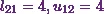 .
.
Thus the value of  will be
![\[(4)(4) + l_{22} = 2.\]](https://appassets.softecksblog.in/engineering_mathematics/assets/em2/12_files/image034.webp)
This means

Next, comes the element from the second row and the third column.
So it will be
![\[l_{21}u_{13} + l_{22}u_{23}=3.\]](https://appassets.softecksblog.in/engineering_mathematics/assets/em2/12_files/image036.webp)
From equations (3), (4) and (5), I can already say  .
.
Thus the value of  will be
![\[(4)(-1) + (-14) u_{23} = 3.\]](https://appassets.softecksblog.in/engineering_mathematics/assets/em2/12_files/image039.webp)
This means

Now comes the third row.
STEP 4
First comes the element from the third row and the first column.
(7) 
Next comes the element from the third row and the second column.
So it will be
![\[l_{31}u_{12} + l_{32} = -3.\]](https://appassets.softecksblog.in/engineering_mathematics/assets/em2/12_files/image042.webp)
From equations (2) and (7), I can already say 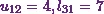 .
.
Thus the value of  will be
![\[(7)(4) + l_{32} = -3.\]](https://appassets.softecksblog.in/engineering_mathematics/assets/em2/12_files/image045.webp)
This means

At the end comes the element from the third row and the third column.
So it will be
![\[l_{31}u_{13} + l_{32}u_{23} + l_{33} = 2.\]](https://appassets.softecksblog.in/engineering_mathematics/assets/em2/12_files/image047.webp)
From equations (3), (6), (7) and (8) I can already say 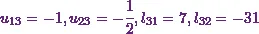 .
.
Thus the value of  will be
![\[(7)(-1) +(-31)\left(-\frac{1}{2}\right) + l_{33} = 2.\]](https://appassets.softecksblog.in/engineering_mathematics/assets/em2/12_files/image050.webp)
This means

Now I’ll use equations (1) – (9) to write the matrices and .
Thus it will be
![\[ \textbf{L} = \begin{pmatrix} 1&0&0\\ 4 &-14&0\\ 7 &-31 &-\frac{13}{2} \end{pmatrix} \]](https://appassets.softecksblog.in/engineering_mathematics/assets/em2/12_files/image052.webp)
and
![\[ \textbf{U} = \begin{pmatrix} 1&4&-1\\ 0 &1 &-\frac{1}{2}\\ 0 &0 &1 \end{pmatrix} .\]](https://appassets.softecksblog.in/engineering_mathematics/assets/em2/12_files/image053.webp)
STEP 5
Now I’ll choose .
Here the matrix will be
So I can say
Now I’ll solve for .
Thus it will be
![\[ \begin{pmatrix} 1&0&0\\ 4 &-14&0\\ 7 &-31 &-\frac{13}{2} \end{pmatrix} \begin{pmatrix} y_1\\ y_2\\ y_3 \end{pmatrix} = \begin{pmatrix} -2\\ -1\\ -18 \end{pmatrix}. \]](https://appassets.softecksblog.in/engineering_mathematics/assets/em2/12_files/image054.webp)
Next I’ll do the matrix multiplication on the left-hand-side.
Therefore it will look like
![\[ \begin{pmatrix} y_1\\ 4y_1 - 14y_2\\ 7y_1 -31y_2 - \frac{13}{2}y_ 3 \end{pmatrix} = \begin{pmatrix} -2\\ -1\\ -18 \end{pmatrix}. \]](https://appassets.softecksblog.in/engineering_mathematics/assets/em2/12_files/image055.webp)
So I get three equations now.
(10) 
Next equation is
![\[4y_1 - 14y_2 = -1.\]](https://appassets.softecksblog.in/engineering_mathematics/assets/em2/12_files/image057.webp)
Using equation (10), I can say that
![\[4(-2) - 14y_2 = -1.\]](https://appassets.softecksblog.in/engineering_mathematics/assets/em2/12_files/image058.webp)
(11) 
The last equation is
![\[7y_1 - 31y_2 - \frac{13}{2}y_3 = -18.\]](https://appassets.softecksblog.in/engineering_mathematics/assets/em2/12_files/image060.webp)
Using equations (10) and (11), I can say that
![\[7(-2) - 31\left(- \frac{1}{2}\right) - \frac{13}{2}y_3 = -18.\]](https://appassets.softecksblog.in/engineering_mathematics/assets/em2/12_files/image061.webp)
(12) 
So I can say
![\[ \begin{pmatrix} y_1\\ y_2\\ y_3 \end{pmatrix} = \begin{pmatrix} -2\\ - \frac{1}{2}\\ 3 \end{pmatrix}. \]](https://appassets.softecksblog.in/engineering_mathematics/assets/em2/12_files/image063.webp)
STEP 6
Now I’ll solve for using the relation .
From Step 4, I already know that the matrix is
Thus it will be
![\[ \begin{pmatrix} 1&4&-1\\ 0 &1 &-\frac{1}{2}\\ 0 &0 &1 \end{pmatrix}\begin{pmatrix} x_1\\ x_2\\ x_3 \end{pmatrix} = \begin{pmatrix} -2\\ - \frac{1}{2}\\ 3 \end{pmatrix}.\]](https://appassets.softecksblog.in/engineering_mathematics/assets/em2/12_files/image064.webp)
Again I’ll use matrix multiplication on the left-hand-side.
Therefore it will be
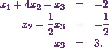
![\[ \begin{pmatrix} x_1&4x_2&-x_3\\ 0 &x_2 &-\frac{1}{2}x_3\\ 0 &0 &x_3 \end{pmatrix} = \begin{pmatrix} -2\\ - \frac{1}{2}\\ 3 \end{pmatrix}.\]](https://appassets.softecksblog.in/engineering_mathematics/assets/em2/12_files/image065.webp)
Like Step 5, here again I get three equations like
From the last equation, I already know that  .
.
From the middle equation, I can say that 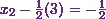 .
.
This gives 
The first equation gives 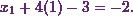
This means 
Hence I can conclude that by using the triangular decomposition method in 3 × 3 matrices I get the solution of the set of equations as
![\[ \begin{pmatrix} x_1\\ x_2\\ x_3 \end{pmatrix} = \begin{pmatrix} -3\\ 1\\ 3 \end{pmatrix}.\]](https://appassets.softecksblog.in/engineering_mathematics/assets/em2/12_files/image072.webp)
This is the answer to the given example.