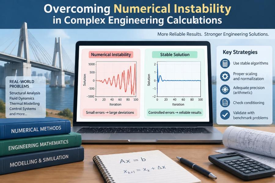

A simulation finishes in seconds, produces six decimal places, and looks reassuringly precise. Then the same model is run with a slightly finer mesh, a different solver tolerance, or a reordered set of equations—and the predicted stress, temperature, or displacement changes dramatically.
That experience is not always evidence that the physics has changed. Often, it is a sign that the calculation has become numerically unstable: small computational imperfections are being amplified until they overwhelm the answer engineers actually need.
Numerical instability appears in spreadsheet estimates, embedded control systems, finite element models, computational fluid dynamics, structural dynamics, and optimization. It can make a plausible result unreliable without producing an obvious error message.
The practical goal is not to eliminate every rounding error. That is impossible. The goal is to design calculations so that unavoidable errors remain small, visible, and controlled.
🧭 What Numerical Instability Really Means
Numerical instability occurs when small disturbances in a computation grow excessively as the calculation proceeds. Those disturbances may come from decimal rounding, uncertain input data, approximation formulas, or the algorithm used to solve a model.
A stable calculation keeps such disturbances bounded or reduces them. An unstable one can turn a tiny difference in an intermediate value into a large difference in the final result.
This is distinct from a model being physically wrong. A perfectly sensible engineering model can still be solved poorly, while a stable numerical result can faithfully represent a poor physical model. Both questions must be checked.
🔍 Why More Digits Do Not Guarantee Accuracy
Computers display many digits, but displayed precision is not the same as trustworthy precision. A result such as 12.483917 may contain only a few meaningful digits if its inputs, equations, or numerical method are sensitive.
Most digital systems store real numbers in finite binary formats. Many simple decimal values cannot be represented exactly, so the stored number is a close approximation. Each operation may add a very small rounding error.
Usually this is harmless. Trouble begins when an algorithm repeatedly magnifies those tiny discrepancies, or when it subtracts nearly equal values and discards the useful information.
🧩 Separate the Four Main Sources of Error
Diagnosing a suspicious answer is easier when errors are separated by origin. They interact, but they require different remedies.
| Source | What it means | Typical response |
|---|---|---|
| Data uncertainty | Inputs are measured or estimated imperfectly. | Improve measurements; report ranges. |
| Model error | The equations simplify real behavior. | Revise assumptions; validate physically. |
| Discretization error | A continuous problem is approximated by finite steps or elements. | Refine mesh or time step systematically. |
| Round-off and algorithmic error | Finite arithmetic and solution procedures distort the calculation. | Use stable formulations and solvers. |
Calling every disagreement “numerical error” hides the real cause. For example, mesh refinement cannot fix an uncertain material property, and higher precision cannot repair an invalid boundary condition.
⚖️ Conditioning: Sensitivity Built Into the Problem
Conditioning describes how strongly the true solution changes when the input changes slightly. It is a property of the mathematical problem, not merely the software.
Consider finding the intersection of two almost parallel lines. A tiny change in either slope can move the intersection a long distance. The calculation is sensitive because the underlying geometry is sensitive.
Ill-conditioned problems are not necessarily unusable. They demand honest input uncertainty, careful scaling, and an awareness that a highly precise output may not be justified.
🛠️ Stability: Sensitivity Introduced by the Method
Stability concerns the numerical method. A well-conditioned problem can be handled unstably if the chosen algorithm amplifies round-off or truncation errors.
For time-dependent equations, a method may be stable only when the time increment is below a limit related to wave speed, diffusion rate, or mesh spacing. Exceeding that limit can produce oscillations or values that grow without physical cause.
Conditioning asks, “Is the problem inherently sensitive?” Stability asks, “Does this computational route control errors?” Engineers need to consider both.
📏 Scaling Is an Early and Powerful Defense
Equations behave better when variables and coefficients have comparable numerical sizes. Mixing a displacement measured in micrometres with a stiffness in gigapascals and a length in kilometres can create coefficients spread across many orders of magnitude.
That spread makes loss of precision more likely and can slow or confuse iterative solvers. It may also make a solver’s default tolerance meaningless: an absolute residual that is tiny for one variable may be large for another.
Use consistent units, nondimensional variables where appropriate, or reference scales such as characteristic length, pressure, velocity, and temperature. Scaling does not change the physics; it makes the arithmetic easier to manage.
➖ Catastrophic Cancellation and Lost Significant Digits
Catastrophic cancellation occurs when two nearly equal numbers are subtracted. Their leading digits cancel, leaving a result whose few remaining digits may be dominated by prior rounding error.
Suppose a calculation subtracts 10.0000012 from 10.0000011. The true difference is small, but any uncertainty in the seventh decimal place now matters enormously relative to the answer.
Look for algebraic rearrangements. Expressions involving differences of close square roots, exponentials, or trigonometric values often have equivalent forms that avoid the risky subtraction. A symbolic rewrite can be more effective than simply using more decimal places.
🔢 Floating-Point Arithmetic Has Practical Limits
Standard double-precision arithmetic is sufficient for a great deal of engineering work, but it is not infinite precision. Very large and very small values can overflow or underflow, and adding a tiny number to a much larger one may leave the stored value unchanged.
Do not assume a calculation fails only when it returns “not a number.” Loss of significance can occur quietly long before overflow.
Higher-precision arithmetic can be useful for reference calculations, exceptionally sensitive subproblems, or verification. It is not a substitute for stable equations: an unstable recurrence can still amplify errors at any precision.
🧮 Summation Order Can Change a Result
In exact arithmetic, addition is associative: the grouping does not matter. In floating-point arithmetic, it can. Adding a long sequence from smallest magnitude to largest often preserves small contributions better than adding them after a large total has already formed.
This matters in energy sums, force assembly, statistical moments, and parallel computations where terms may be combined in different orders. Small differences are expected, but large differences indicate sensitivity worth investigating.
For demanding sums, compensated summation techniques retain a correction for lost low-order digits. The wider lesson is simple: operations that look algebraically interchangeable may not be numerically interchangeable.
📐 Near-Singular Matrices Cause Fragile Linear Systems
Many engineering models become a linear system, commonly written as Ax = b. If the matrix A is singular, no unique solution exists. If it is nearly singular, a solution may exist but react sharply to tiny perturbations.
In structural analysis, this can happen when a model has an unintended rigid-body mode because a support constraint is missing. In circuit or flow models, it may indicate a disconnected reference, redundant relation, or nearly dependent equations.
A solver warning about poor conditioning is not merely a software nuisance. It may expose a modeling mistake, an extreme scale mismatch, or a system that genuinely cannot identify the requested quantity reliably.
🏗️ Pivoting Protects Direct Linear Solvers
Gaussian elimination solves many linear systems efficiently, but dividing by a very small pivot can magnify round-off error. Pivoting reorders rows, and sometimes columns, to choose safer pivots.
Modern numerical libraries generally implement suitable pivoting automatically. Problems arise when engineers hand-code elimination, disable safeguards for convenience, or form equations in a way that creates avoidable small pivots.
Use established linear algebra routines rather than custom matrix inversion. In most cases, solving Ax = b directly is more accurate and efficient than explicitly calculating A⁻¹ and multiplying it by b.
🔁 Iterative Solvers Need More Than a Stop Button
Large sparse models often use iterative methods, which improve an estimated solution step by step. Their performance depends on matrix properties, initial guesses, scaling, and preconditioning.
A residual measures how well the current estimate satisfies the equations. A small residual is useful evidence, but it does not automatically mean the solution error is small, especially in an ill-conditioned system.
Set stopping criteria using both relative and absolute measures when appropriate. Also monitor iteration counts and trends: a solver that suddenly needs far more iterations after a model change may be revealing a numerical or physical issue.
🧱 Preconditioning Changes the Difficulty, Not the Physics
A preconditioner transforms a linear system into an equivalent form that iterative solvers can handle more efficiently. Ideally, it clusters the difficult numerical behavior without changing the desired solution.
Good preconditioning can reduce solve time substantially and improve robustness. However, its effectiveness can depend on mesh quality, material contrasts, contact conditions, and the evolving state of a nonlinear model.
Treat preconditioner choice as part of the computational design. A method that works on a small benchmark may be unsuitable for a larger, more heterogeneous production model.
⏱️ Time-Step Size Can Create Nonphysical Behavior
In transient heat transfer, vibration, fluid flow, and control simulation, the time step determines what changes the calculation can resolve. An overly large step may miss sharp events, damp oscillations incorrectly, or destabilize an explicit method.
An excessively small step is not automatically better. It increases cost, can accumulate round-off through many operations, and may make a poorly posed model look busy rather than accurate.
Run a time-step convergence check. Compare key outputs at progressively smaller steps and look for a stable trend, not simply a simulation that completes without warnings.
🌊 Explicit and Implicit Methods Make Different Trade-Offs
Explicit time integration computes the next state directly from the current one. It is straightforward and can be efficient per step, but it often has a strict stability limit.
Implicit methods solve a coupled system at each step. They can permit larger stable steps for many problems, particularly diffusion-like behavior, but each step is more expensive and may introduce numerical damping or nonlinear convergence challenges.
“Unconditionally stable” in a mathematical sense does not mean “accurate at any time step.” A large implicit step can remain bounded while smoothing or shifting behavior that matters to the engineering decision.
🕸️ Mesh Quality Influences More Than Visual Detail
Finite element and finite volume meshes turn geometry into discrete cells or elements. Highly skewed, stretched, inverted, or abruptly changing elements can degrade matrix conditioning and local approximation quality.
A finer mesh near a stress concentration may be necessary, but blindly refining everywhere can make the system larger and harder to solve while leaving the critical poor-quality region unchanged.
Inspect mesh metrics, refine based on solution features, and check whether important outputs converge. Mesh independence means the decision-relevant result changes negligibly over further sensible refinement; it does not mean every local value is exact.
📍 Singularities Need Engineering Interpretation
Some models contain mathematical singularities. A perfectly sharp re-entrant corner, a point load, or an idealized contact edge can produce stresses that grow as the mesh becomes finer.
That trend is not necessarily solver failure. It may mean the idealization asks for a pointwise stress that the continuum model cannot represent as a finite value.
Replace the idealization with a realistic load distribution or fillet when justified, or evaluate quantities that remain meaningful, such as averaged stress away from the singular point, force transfer, displacement, or an energy-based measure.
🧪 Nonlinear Problems Can Follow the Wrong Path
Material plasticity, large deformation, contact, chemical reactions, and turbulent closures commonly create nonlinear equations. A nonlinear solver may converge to different valid solution branches depending on initial conditions, load increments, and constraints.
Sudden jumps, alternating states, or failure to reduce the residual can signal that the load step is too large, the tangent information is poor, or the problem has genuine physical instability.
Use continuation: increase load or another control parameter gradually, carry forward a credible previous solution, and record convergence behavior. Smaller increments are a diagnostic tool, not a universal cure.
🎛️ Regularization Can Stabilize an Ill-Posed Task
Inverse problems infer causes from effects: estimating a heat source from temperature measurements, identifying material parameters, or reconstructing a load from displacement data. These tasks can be ill-posed because many input patterns explain nearly the same observations.
Regularization adds a justified preference, such as smoothness, small parameter changes, or physically plausible bounds. It reduces sensitivity to measurement noise.
The trade-off is bias. Strong regularization may produce a stable but overly smooth answer. Choose its strength based on measurement uncertainty, physical knowledge, and sensitivity checks rather than treating it as a hidden solver setting.
📊 Residuals, Errors, and Validation Are Different Tests
A residual checks the algebraic equations. An error compares the computed state with the exact state, which is usually unknown. Validation compares model predictions with real observations or trusted reference data.
These are related but not interchangeable. A CFD model can have a very low algebraic residual and still predict the wrong pressure loss because boundary conditions, turbulence assumptions, or geometry details are inadequate.
Use the strongest available comparison: an analytical benchmark, a manufactured solution, a hand calculation for a simplified case, measured data, or a second independently implemented method.
🧷 Conservation Laws Are Valuable Numerical Alarms
Mass, charge, momentum, and energy balances provide powerful checks because they reflect physical structure rather than a solver’s internal status. A solution may look smooth and still leak mass or create energy numerically.
Track global balances and, where relevant, local fluxes. Define a residual in physically meaningful units so a discrepancy can be compared with expected loads, source terms, and measurement uncertainty.
A small imbalance may be acceptable depending on discretization and tolerance. The key is to quantify it and decide whether it is small relative to the conclusion being drawn.
🔄 Reproducibility Helps Reveal Hidden Sensitivity
If repeating the same calculation produces materially different answers, investigate random seeds, parallel reduction order, adaptive meshing decisions, and uninitialized variables. Some small variation is normal in large parallel floating-point computations.
The concern is whether that variation changes a design choice or physical interpretation. Preserve input files, solver versions, mesh-generation settings, tolerances, and post-processing steps so differences can be traced.
Reproducibility is not administrative overhead. It is a numerical diagnostic that makes unexpected variation visible rather than anecdotal.
🧾 Report Precision Honestly
Output formatting should reflect what the analysis can support. Reporting a safety margin to six decimal places is misleading if material properties, loads, or boundary conditions are uncertain at much larger scales.
Keep extra digits internally where they help computation, but round reported values sensibly. Pair critical results with assumptions, convergence evidence, and uncertainty ranges when the application requires them.
Honest precision improves decisions because it focuses attention on meaningful differences rather than numerical decoration.
🚩 Common Responses That Usually Make Things Worse
When a calculation misbehaves, several tempting actions can hide the underlying problem.
- Increasing iterations blindly: useful only if the method is converging toward a meaningful solution.
- Refining the mesh without a plan: may expose a singularity or increase solver difficulty without improving the relevant output.
- Relaxing tolerances immediately: can make a run finish while accepting an inadequate solution.
- Adding artificial damping: may suppress numerical oscillations but also remove real dynamics.
- Trusting a single plot: visually smooth contours do not demonstrate conservation, convergence, or physical validity.
Each tool has legitimate uses. The mistake is applying it before identifying whether the issue is conditioning, stability, formulation, data, or physics.
🧰 A Practical Diagnostic Workflow
Use a repeatable process when outputs seem fragile. It reduces guesswork and makes findings easier to communicate.
- Check units, signs, boundary conditions, and orders of magnitude with a simplified hand estimate.
- Inspect warnings, residual histories, conservation balances, and solver iteration counts.
- Rescale variables and identify coefficients or states with extreme magnitude differences.
- Vary one numerical choice at a time: mesh, time step, tolerance, solver, or precision.
- Compare decision-relevant outputs, not only maximum local values.
- Test against a benchmark, an alternate formulation, or measured behavior where available.
- Document what changes the answer and what does not.
This sequence does not guarantee a perfect model. It creates evidence for whether a result is numerically dependable enough for its intended use.
🧠 Choose the Method to Fit the Question
The best numerical approach depends on what must be predicted. A coarse model may be adequate for total heat duty but inadequate for peak thermal stress. A steady solution may support a long-term operating estimate but not a transient safety assessment.
Define acceptance criteria before running the full calculation. Examples include a bounded change in total force under mesh refinement, conservation within a specified engineering tolerance, or a stable predicted operating regime under reasonable parameter variation.
This avoids spending computation on irrelevant precision while ensuring that numerical effort is concentrated on quantities that drive decisions.
🤝 Numerical Judgment Combines Mathematics and Engineering
Robust calculation is not achieved by a single setting or software package. It requires mathematical awareness, physical judgment, and disciplined verification.
Ask practical questions throughout: Does the magnitude make sense? Is the trend physically plausible? Which assumption dominates uncertainty? Would a modest change in resolution alter the decision?
These questions turn numerical analysis from a black-box activity into an engineering process that can be reviewed, repeated, and trusted appropriately.
✅ The Core Principle: Control Error Before Interpreting Results
Numerical instability is manageable when it is treated as an engineering risk rather than an obscure software defect. Start by distinguishing inherent sensitivity from unstable computation, then use scaling, sound formulations, suitable solvers, and systematic convergence checks.
Do not demand certainty where the model or data cannot provide it. Instead, establish whether the result is stable enough, accurate enough, and transparent enough for the decision at hand.
The strongest calculations are not those with the most digits. They are the ones whose limitations have been tested, understood, and communicated.
Reliable engineering calculations come from controlling how errors enter, grow, and influence the final decision—not from trusting a precise-looking number. 📐🔍⚙️