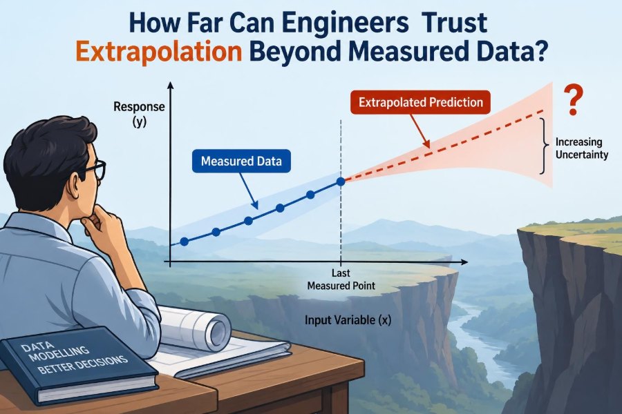

A test rig produces a clean set of measurements. A material’s strength rises predictably with temperature over the range tested, a pump curve is smooth, and a fitted equation has an impressive match to the data. The tempting next step is to extend the curve a little farther.
That step is often necessary. Engineers must estimate aircraft loads beyond a wind-tunnel campaign, battery life beyond a short trial, flood levels beyond recorded storms, and machine wear beyond the first months of service.
But a model that describes what has been observed is not automatically a model of what happens next. Beyond the measured range, the question changes from “Does this fit?” to “What physical behavior are we assuming?”
Extrapolation is therefore not a mathematical sin or a shortcut to avoid. It is a disciplined prediction under uncertainty—and it becomes trustworthy only when mathematics, physics, evidence, and consequences are considered together.
📏 What Extrapolation Actually Means
Extrapolation estimates an output outside the range of available observations. If a sensor has recorded a bridge’s deflection under loads from 0 to 200 kN, estimating deflection at 250 kN is extrapolation.
This differs from interpolation, which estimates between known points. Interpolation can still be wrong, but nearby measurements constrain it on both sides. Extrapolation has no such boundary on the unknown side.
🧩 A Good Fit Is Not a Future Guarantee
A curve can pass close to every measured point and still fail immediately beyond the last one. Regression measures agreement with the sample, not a promise that the same relationship continues.
For example, a quadratic fitted to three points can bend sharply upward or downward outside them. The calculation is valid; the implied behavior may not be.
🔍 The Central Question: What Mechanism Continues?
The strongest basis for extrapolation is a reason to believe the governing mechanism remains unchanged. A simple linear thermal expansion relation is more defensible over a modest extension of temperature if the material stays in the same phase and stress state.
It is much less defensible if the extension approaches yielding, creep, oxidation, melting, or a change in microstructure. The relevant limit is not merely “beyond the data”; it is often “before the next mechanism appears.”
🗺️ Measured Range Versus Operating Envelope
Always distinguish the calibration range from the intended operating envelope. A model calibrated at mild ambient temperatures may be used in a product that sees cold starts, high internal heat, vibration, dust, and variable supply voltage.
One input may remain in range while another does not. A turbine performance model, for instance, can be extrapolated by speed, pressure ratio, inlet temperature, or several variables simultaneously. Its practical distance from evidence is multidimensional.
📈 Why Straight Lines Become Risky
Linear extrapolation is appealing because it is transparent. If a quantity changes by 2 units per input unit across the test interval, extending the line feels reasonable.
Yet many engineering relationships are only locally linear. Springs can become nonlinear near geometric limits, sensors can saturate, friction can change with lubrication regime, and heat loss often changes as temperature differences grow.
A straight line is best regarded as a local approximation, not a default law of nature.
➿ Curved Fits Can Be Even More Fragile
High-order polynomials can produce excellent in-range fits while behaving wildly outside the data. Small uncertainty in their coefficients may become a large change at the extrapolated input.
A smooth curve also looks persuasive to the eye. That visual smoothness should not be confused with physical credibility. Unless the shape follows a justified model, a flexible fitted curve is usually a poor long-range predictor.
⚙️ Physics-Based Models Earn More Trust
A physics-based model starts from conservation laws, material behavior, geometry, and boundary conditions. It may still contain uncertain parameters, but its response is constrained by known relationships.
For example, a heat-transfer model based on energy balance can be extrapolated more responsibly than a purely empirical temperature-versus-time curve, provided the assumed heat-transfer modes and material properties remain applicable.
This does not make physics models infallible. Incorrect boundary conditions, omitted failure modes, or uncertain properties can dominate their error.
🧪 Empirical Models Have a Clear Boundary
Empirical models learn a relationship directly from observations: a fitted fatigue curve, a pump map, or a correlation for pressure drop. They are often extremely useful inside the conditions represented by their data.
Outside that domain, the model may be asked to answer a question it was never designed to answer. Documenting its valid inputs is not administrative overhead; it is part of the model itself.
🧱 Regime Changes Break Familiar Trends
A regime change occurs when the dominant behavior changes. Flow can transition from laminar to turbulent, a material can yield, a battery can enter a different degradation pathway, or a control system can hit an actuator limit.
At these boundaries, a trend may change slope, flatten, reverse, or become unstable. A modest-looking extrapolation can cross a regime boundary if the measured data ended near one.
🌡️ Thresholds and Discontinuities Matter
Some changes are gradual; others are abrupt. A thermostat switches, a valve opens, a protective controller derates power, or a crack begins to propagate rapidly after a critical condition is reached.
Curve fitting is weakest when it silently smooths over thresholds. Engineers should identify known triggers and represent them explicitly rather than expecting one continuous equation to capture everything.
📊 Noise Does Not Reveal the Whole Uncertainty
Repeated measurements reveal random variation, such as sensor noise or test-to-test scatter. That information is valuable, but it does not capture model-form error: the possibility that the equation itself has the wrong structure.
A narrow confidence interval around a fitted line can create false comfort. It often describes uncertainty in the fitted parameters under the model’s assumptions, not uncertainty about whether the model remains valid outside the sample.
🎯 Prediction Intervals Are More Honest Than Single Values
When extrapolation is necessary, report a range rather than only a central estimate. A prediction interval expresses plausible variation in a future observation, while a confidence interval typically concerns uncertainty in an estimated mean relationship.
Neither interval automatically includes every unknown mechanism. Still, presenting a range encourages decisions based on margins and consequences rather than on an apparently precise single number.
📐 Distance Beyond the Data Is Not One Number
“Only 10% beyond the test range” can be either harmless or hazardous. The meaning depends on the model’s curvature, uncertainty, nearby thresholds, and the scale on which the problem behaves naturally.
For an exponential process, equal steps in the raw variable can have very unequal effects. For logarithmic relationships, the relevant notion of distance may be a ratio rather than an absolute difference.
🔢 Choose Variables That Match the Physics
Sometimes extrapolation improves when the variables are transformed in a physically meaningful way. A decay process may become linear on a logarithmic scale; a dimensionless group may collapse results from different sizes or operating conditions.
Transformations are not cosmetic. They should follow theory or a clear diagnostic purpose. A transformation chosen merely because it straightens a plot can conceal important departures from the assumed mechanism.
🧷 Constraints Prevent Impossible Predictions
Useful models respect known limits. Efficiencies generally have physical bounds, concentrations cannot become negative, and a tank level cannot exceed its geometry without overflow.
Imposing constraints can make an extrapolated estimate less convenient mathematically but more credible operationally. If a fitted model predicts impossible values, treat that as a warning about the model’s domain, not a strange result to explain away.
🏗️ Example: Extending a Load–Deflection Curve
Imagine a beam tested only within its elastic range. The load–deflection graph is linear, so extending it to a higher load may estimate service deflection reasonably if stresses remain below yielding and support conditions do not change.
Using the same line to predict behavior after yielding is different. Plastic deformation changes the relationship; residual deflection and local buckling may become relevant. The measured slope was not a universal property of the beam.
🔋 Example: Predicting Battery Degradation
A battery may show nearly steady capacity loss through an early set of charge cycles. Extending that trend over a longer lifetime can be useful for planning, but temperature, charging rate, storage time, and usage profile can alter the path.
A responsible projection states the assumed duty cycle and treats the result as conditional. “This estimate applies if future conditions resemble the tested conditions” is far more informative than an unqualified lifetime number.
🌊 Example: Designing for Rare Environmental Loads
Flood, wind, and wave design often requires estimating events rarer than those directly observed. Here extrapolation cannot simply be avoided, because infrastructure must address future extremes.
The appropriate response is not blind trust in a fitted tail distribution. It is to combine historical records, physical understanding, uncertainty analysis, conservative design choices, and periodic reassessment as new information becomes available.
🧮 Simulation Does Not Eliminate Extrapolation
Finite-element analysis, computational fluid dynamics, and digital twins can explore conditions that were not physically tested. But simulation itself extrapolates whenever material properties, turbulence closures, contact models, or boundary conditions are used outside their validated range.
Numerical detail is not the same as accuracy. A simulation with millions of elements can still be confidently wrong if its inputs or assumptions are inappropriate.
✅ Validate at the Edge, Not Only the Middle
Validation data concentrated near normal conditions show whether a model works where it is easiest. To assess extrapolation, seek checks near the edge of the intended domain and, when feasible, slightly beyond the routine range.
Hold out edge-case data during development rather than fitting every available point. If a model cannot predict the withheld edge, there is little reason to trust it farther out.
🔄 Use Progressive Extension Tests
A practical approach is progressive extension. Fit a model using an early portion of the available range, predict the next portion, compare with the measurements, then repeat.
This does not prove long-range behavior, but it reveals how prediction error grows as the model moves away from calibration data. It also compares candidate models under the task that matters: forecasting outside a known boundary.
🧠 Perform Sensitivity Analysis
Sensitivity analysis asks how much an output changes when uncertain inputs or parameters are varied. If a small change in a heat-transfer coefficient doubles a projected temperature rise, the extrapolation is fragile.
Focus measurement effort on high-sensitivity quantities. Reducing uncertainty in a parameter that barely affects the decision adds little value, while one critical uncertain assumption may justify a new experiment.
🪜 Add Safety Margins Deliberately
Safety factors and design margins are often necessary when predictions face uncertainty, but they should not become a substitute for understanding. A margin may address ordinary variation while failing to cover a missed regime change.
The right margin depends on consequences, uncertainty, inspectability, redundancy, and the ability to intervene. A consumer comfort estimate and a pressure-vessel limit do not deserve the same tolerance for unknowns.
🚦Let Consequence Set the Evidence Standard
Every extrapolation is not equally consequential. A rough estimate of paint drying time can tolerate a larger error than a prediction of crack growth in a critical component.
| Decision context | Reasonable approach |
|---|---|
| Low consequence, reversible | Use a simple estimate, state assumptions, monitor results. |
| Moderate consequence | Use multiple models, sensitivity checks, and targeted validation. |
| High consequence or hard to reverse | Seek new data, independent review, conservative limits, and explicit failure analysis. |
The point is not to eliminate uncertainty. It is to match the rigor of the evidence to the cost of being wrong.
📝 State Assumptions Where Decisions Are Made
An extrapolated result should travel with its assumptions. If a chart, spreadsheet, or dashboard shows only the answer, later users may apply it under conditions the original analyst never intended.
- State the measured input range and source of data.
- Name the model form and its physical rationale, if any.
- Identify conditions assumed to remain unchanged.
- Report uncertainty and known unmodeled effects.
- Define an action or review point if limits are approached.
🧭 Compare More Than One Plausible Model
If several models fit measured data similarly but diverge outside it, that divergence is useful information. It exposes uncertainty that a single preferred curve would hide.
Compare a simple empirical model, a constrained physical model, and a deliberately conservative scenario when appropriate. The spread is not an embarrassment; it can guide where further data are worth collecting.
🛠️ Design Experiments for the Decision, Not Just the Fit
Testing only where a system is comfortable produces clean data but may leave the decisive region unknown. Experimental plans should include conditions near expected limits, while respecting safety and equipment constraints.
Vary influential inputs separately when possible. Otherwise, two factors that always change together can appear to have one combined effect, making later extrapolation unreliable.
👀 Monitor Reality After Deployment
Even careful pre-deployment analysis cannot capture every field condition. Instrumentation, inspections, alarms, and periodic model updates turn an extrapolation into a managed prediction rather than a one-time guess.
Monitoring should focus on leading indicators: temperatures before overheating, vibration before damage, drift before loss of control, or pressure changes before capacity is compromised.
⚠️ Common Failure: Extending Convenience Trends
A frequent mistake is extrapolating the variable that is easiest to measure rather than the mechanism that governs performance. Another is using average conditions when failures occur in combinations of extremes.
Watch for familiar warning signs: a model predicts negative values, unlimited growth, efficiency above a physical bound, or smooth behavior through a known threshold. These are prompts to revisit assumptions.
🤝 Communicate Uncertainty Without Becoming Vague
“The model may be wrong” is true but unhelpful. Better communication names the uncertainty, its likely direction where known, the affected decision, and the next action.
For example: “Above the tested temperature range, predicted deformation is highly sensitive to creep properties; do not use this estimate as an acceptance limit without elevated-temperature testing.” That is specific, actionable, and appropriately cautious.
🏁 The Core Principle: Extend Evidence, Not Just Curves
Engineers can trust extrapolation to the extent that the conditions, mechanisms, assumptions, and consequences are understood. The graph matters, but the world that created the graph matters more.
Use extrapolation confidently when it is local, physically supported, constrained by known limits, checked against edge data, and paired with uncertainty-aware decisions. Slow down when a threshold, a new regime, or serious consequences lie ahead.
The safest extrapolation is not the one with the smoothest line; it is the one whose assumptions remain credible beyond the last measured point. 📐🔎🛠️