
A bridge designer checks whether a proposed deck will deflect too far under traffic. A process engineer estimates the temperature profile through a reactor. A controls engineer tunes a motor drive that must respond quickly without oscillating.
Each problem is governed by equations, but the equations are rarely neat enough to solve with pencil-and-paper algebra. Material behaviour may be nonlinear, forces may vary with position, and one part of a system may influence another over time.
That is where numerical solvers enter the picture. They do not “discover” an exact hidden answer by magic. They apply carefully chosen approximations, repeatedly, while measuring whether those approximations have become good enough for the engineering decision at hand.
Understanding what happens under the hood helps students use software more intelligently and helps working engineers judge when a polished plot deserves confidence—and when it needs closer inspection.
🧩 Why engineering equations become difficult
Many introductory equations have closed-form solutions: explicit formulas that give the answer directly. For example, a constant-acceleration motion problem can be solved with a few algebraic substitutions.
Real systems often contain nonlinearity, meaning that doubling an input does not simply double an output. Contact forces, large structural deflections, turbulent flow models, chemical reaction rates, and radiation heat transfer commonly behave this way.
Equations also become difficult when they are coupled. Temperature can affect viscosity, viscosity can affect flow, and flow can change temperature. A solver must find values that satisfy all of these relationships together.
🎯 The problem a solver is actually trying to solve
At its core, a numerical solver converts an engineering model into a finite set of arithmetic operations. Its target may be a root, a system of algebraic equations, a differential equation, an optimization problem, or a combination of these.
For a root-finding problem, the goal is to find a value of x for which f(x) = 0. A beam equation might be rearranged into this form when finding the load that produces a specified displacement.
For a system, the solver seeks a vector of unknowns—perhaps pressures at many pipe junctions—such that every governing equation is satisfied within an accepted tolerance.
🗺️ From a physical system to a mathematical model
A solver can only solve the model it is given. Before numerical work begins, an engineer chooses governing laws, assumptions, material properties, geometry, loads, and boundary conditions.
Consider heat conduction through a wall. Fourier’s law relates heat flux to a temperature gradient, but the model still needs wall thickness, thermal conductivity, internal heat generation if present, and temperatures or heat-transfer conditions at the surfaces.
This translation is often more consequential than the eventual solver setting. A highly accurate solution to an inappropriate model is still inappropriate for the physical system.
🚧 Boundary and initial conditions close the problem
Differential equations describe relationships between changing quantities, but they usually do not specify one unique physical situation by themselves. Boundary conditions describe what happens at edges or interfaces; initial conditions describe the state at a starting time.
For a fixed beam, zero displacement and zero rotation are imposed at its support. For transient cooling, the initial temperature field is required before the solver can calculate later temperatures.
Missing, contradictory, or physically unrealistic conditions can make a problem unsolvable or produce a mathematically valid result with no useful physical meaning.
🔢 Discretization turns continua into manageable pieces
Most engineering fields vary continuously in space or time. Numerical computation replaces that continuum with a finite representation, a process called discretization.
A pipe may be divided into axial segments. A plate may be divided into a mesh of small elements. A time history may be represented at discrete instants separated by a time step.
The solver then estimates values—such as temperature, displacement, or velocity—at selected points or within selected regions. The result is not the continuous field itself; it is an approximation whose quality depends partly on how that field was represented.
🕸️ Meshes define where detail can exist
In finite element and computational fluid dynamics models, a mesh partitions the geometry into elements or control volumes. Nodes, element centers, or faces carry the unknown values needed by the method.
A coarse mesh may capture the broad bending of a bracket but miss a sharp stress gradient near a small fillet. A refined mesh can resolve more detail, but it also adds unknowns and increases memory use and runtime.
Mesh quality matters as well as mesh density. Extremely skewed, stretched, or distorted elements can degrade numerical accuracy and make iterative solution more difficult.
📏 Approximation is local before it becomes global
Discretization works by approximating behaviour over small regions. In a finite element model, a displacement field inside each element is represented with shape functions built from nodal values.
In finite differences, derivatives are approximated from values at nearby grid points. The derivative of a quantity is replaced by a difference quotient, which becomes more accurate as spacing decreases under suitable conditions.
These local approximations assemble into one global model. Their individual errors do not simply vanish; engineers must check whether their combined effect is acceptably small for the quantity they care about.
🧮 Residuals measure unsatisfied equations
Once the model is assembled, a trial solution can be substituted back into its governing equations. The remaining imbalance is called a residual.
If a nodal force balance says applied force should equal internal force, their difference is a residual. If an iterative fluid solution has nonzero mass imbalance in a control volume, that imbalance is also reflected in residual behaviour.
Small residuals are usually desirable because they indicate that the discrete equations are being satisfied. They do not, by themselves, prove that the discrete equations accurately represent the real physical system.
🔁 Iteration improves an initial guess
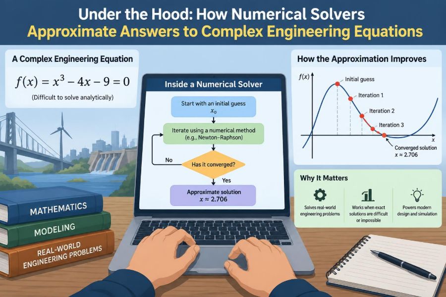
For many problems, especially nonlinear ones, the solver begins with an initial guess and improves it through repeated updates. One cycle of estimate, evaluate, and correct is an iteration.
Imagine estimating a pipe-flow rate. A guessed flow rate gives a pressure-loss estimate; the pressure-loss mismatch suggests a revised flow rate. The solver repeats this cycle until the mismatch is small enough.
A useful initial guess can reduce computation substantially. A poor one may slow convergence, lead to an unintended solution branch, or cause the algorithm to fail.
📍 Bisection: slow, steady root finding
The bisection method finds a root inside an interval where a continuous function changes sign. It evaluates the midpoint, retains the half-interval that still brackets the sign change, and repeats.
Its major strength is reliability: if its assumptions hold and the interval truly brackets one or more roots, the interval shrinks predictably. Its drawback is that convergence is comparatively slow.
For a hypothetical calibration equation where a sensor offset is known to lie between two values, bisection provides a dependable baseline. It is especially useful when function evaluations are inexpensive and robustness matters more than speed.
⚡ Newton’s method uses slope information
Newton’s method improves a root estimate by following the local tangent line. In one variable, it uses both the function value and its derivative to calculate a new estimate.
Near a well-behaved root, Newton’s method can converge very quickly. That speed explains its popularity in nonlinear structural analysis, circuit simulation, and many multiphysics calculations.
It can also misbehave. A derivative near zero, a poor initial guess, or a strongly nonlinear function may send an update far from the desired root. Practical solvers often limit step size or switch strategies when this occurs.
🧠 Jacobians organize coupled nonlinear systems
For multiple unknowns, Newton-like methods use a Jacobian: a matrix of partial derivatives showing how each equation changes when each unknown changes.
In a network with pressures and flows, one variable can influence several equations. The Jacobian captures those sensitivities and allows the solver to calculate coordinated updates rather than adjusting one variable blindly at a time.
Building and factoring a Jacobian may be expensive for large models. Software may use analytically derived derivatives, numerical approximations, automatic differentiation, or methods that approximate the Jacobian to balance cost and robustness.
🏗️ Linear systems appear everywhere
After discretization—or after linearizing a nonlinear model—a problem often takes the form Ax = b. Here, x contains unknown values, A describes how they interact, and b represents loads, sources, or known conditions.
A finite element stiffness matrix is a familiar example. Each row expresses equilibrium associated with a degree of freedom, while off-diagonal terms capture how one location influences another.
Even when the original physics is nonlinear, each iteration may require solution of a linear system. Consequently, efficient linear algebra is central to practical numerical engineering.
🧱 Direct solvers and iterative solvers differ
Direct methods, such as matrix factorization, transform a linear system through a prescribed sequence of operations. Given enough memory and stable arithmetic, they can produce a solution in a predictable way.
Iterative methods generate a sequence of improving estimates. They are often attractive for very large sparse systems, where most matrix entries are zero and storing a dense matrix would be wasteful.
| Approach | Useful when | Practical trade-off |
|---|---|---|
| Direct linear solver | System size is moderate or repeated reliability is needed | Can require substantial memory and factorization work |
| Iterative linear solver | System is large, sparse, and suitably conditioned | Performance depends strongly on scaling and preconditioning |
Neither approach is universally superior. Matrix structure, hardware, required accuracy, and the number of repeated solves all influence the choice.
🧰 Preconditioning makes iterations practical
An iterative solver may converge slowly when the equations are poorly scaled or when the matrix has an unfavourable structure. A preconditioner transforms the problem into one that is easier for the iteration to solve.
It does not change the intended physical solution; ideally, it changes only the route taken to reach it. A useful analogy is choosing a better coordinate system before measuring a complicated shape.
Preconditioner design is a technical subject in itself. An elaborate preconditioner may cut iteration count but consume more setup time, so the fastest overall workflow is not always the one with the fewest iterations.
⏱️ Time stepping moves transient models forward
When a system changes over time, the solver advances from one time level to the next. This is called time integration or time stepping.
For a cooling component, each step uses the current temperature field to estimate a later field. Smaller time steps usually capture rapid changes more faithfully, but they require more calculations.
The selected time step is therefore a modelling decision, not merely a software preference. A step suitable for slow thermal diffusion may be far too large for a rapidly switching electrical circuit.
⚖️ Explicit and implicit schemes trade cost for stability
An explicit scheme computes the next state mainly from known current information. It is conceptually straightforward and can be efficient per step, but it often requires very small time steps to remain stable.
An implicit scheme includes unknown future-state information, so each time step requires solving equations. That added work can permit larger stable steps for many diffusion-dominated or stiff problems.
Stability is not the same as accuracy. An implicit calculation may remain numerically stable with a large step while smoothing out short-lived behaviour that the engineering question actually requires.
🪨 Stiffness has a special numerical meaning
A system is called stiff when it contains processes evolving on very different time scales. Chemical kinetics can include both fast reactions and slow changes; mechanical systems can include high-frequency vibration alongside gradual motion.
Stiffness can force explicit methods to take steps dictated by the fastest process, even if the analyst is mainly interested in the slow one. Implicit methods are often considered for this reason.
The term should not be confused with material stiffness, although both ideas arise frequently in engineering. Numerical stiffness concerns the difficulty of advancing an equation in time.
🎛️ Tolerances decide when “close enough” is enough
No numerical computation is exact. Solvers stop according to criteria such as residual size, change between iterations, estimated local time-integration error, or a maximum iteration count.
Absolute tolerance sets a fixed permitted magnitude; relative tolerance scales the requirement with the size of the variable or residual. Using only one can be misleading when a model contains values with very different magnitudes.
Tolerances should relate to the question. Requiring pressure accuracy far below uncertainty in the input roughness or boundary data may add runtime without improving a meaningful engineering conclusion.
📉 Convergence is evidence, not a certificate of truth
When a solver converges, it has met its specified numerical stopping criteria. This is useful evidence that the algorithm has solved the discretized equations consistently.
Convergence does not automatically establish correct geometry, realistic loads, appropriate turbulence closure, valid constitutive data, or sufficient mesh resolution. These are separate sources of uncertainty.
A converged result can also represent the wrong equilibrium state in a nonlinear problem. Inspecting deformation patterns, balances, and expected physical trends remains essential.
🔍 Verification asks whether the equations were solved right
Verification examines the numerical implementation and solution process. Typical checks include mesh refinement, time-step refinement, conservation balances, comparison with a simpler analytical case, and inspection of residual histories.
For example, if halving characteristic mesh spacing produces little change in the displacement at a point of interest, that result is more credible than one obtained from a single arbitrary mesh.
Verification does not require a perfect reference solution. It asks whether numerical error is controlled well enough to support the intended use of the model.
🧪 Validation asks whether the model represents reality
Validation is different: it compares model predictions with relevant physical observations or trusted experimental data. A correctly implemented heat-transfer model can still be invalid for a situation where an overlooked contact resistance dominates behaviour.
Validation should use conditions relevant to the intended application. Agreement in one operating range does not necessarily justify extrapolation to much higher load, temperature, speed, or geometric scale.
When data are limited, engineers should state that limitation plainly and avoid treating a numerical output as a measured fact.
📐 Grid independence needs a quantity of interest
“The mesh is fine enough” is incomplete unless it identifies what must be accurate. Global pressure drop, maximum von Mises stress, lift coefficient, and peak temperature can respond very differently to mesh refinement.
Stress near an idealized sharp re-entrant corner may increase as the mesh is refined because the mathematical model has a stress singularity. In that case, reporting a single peak stress without interpretation can be misleading.
Choose a quantity of interest, refine where gradients matter, and examine whether that quantity changes systematically. The right mesh is tied to the decision, not just to an attractive element count.
🧯 Singularities and discontinuities need careful interpretation
Some model features create abrupt changes or unbounded idealized values. Point loads, perfectly sharp corners, rigid constraints, shocks, and material interfaces can challenge standard numerical assumptions.
Refining near a true mathematical singularity does not necessarily produce a finite peak. Instead, engineers may assess forces, averaged stresses over a meaningful area, energy measures, or a more realistic geometric representation.
This is a reminder that numerical detail is not automatically physical detail. A bright contour hotspot should prompt a question about modelling assumptions before it drives a redesign.
💻 Floating-point arithmetic has limits
Computers store most real numbers with finite precision. Values are rounded, and repeated operations can accumulate small numerical errors. Very large and very small quantities in the same calculation can make this more troublesome.
Subtracting nearly equal values can lose meaningful digits, while ill-conditioned systems can amplify tiny changes in inputs or arithmetic. These effects are not usually visible in a final dashboard.
Scaling variables to comparable magnitudes, using appropriate units, and avoiding unnecessarily extreme tolerances can improve numerical behaviour. More decimal places in output do not create more physical certainty.
📊 Conditioning reveals sensitivity in the equations
A problem is well-conditioned when small input changes produce relatively small output changes. It is ill-conditioned when tiny changes in data, rounding, or modelling assumptions can cause large solution changes.
For example, nearly redundant equations or nearly singular structural constraints can make a matrix difficult to solve reliably. The issue may arise from the physical setup, the chosen variables, or an accidental modelling error.
Solver warnings about conditioning deserve investigation. They can signal a need to rescale the model, revise constraints, improve measurements, or acknowledge that the requested prediction is inherently sensitive.
🧭 Nonlinear problems may have multiple answers
Some nonlinear systems admit more than one equilibrium or operating state. A buckling structure may have distinct deformed configurations, and a nonlinear circuit can have different steady states under the same nominal conditions.
The path taken by the solver matters. Load stepping, continuation methods, and carefully chosen initial conditions can help trace a physically relevant branch rather than jumping unpredictably between solutions.
When multiple solutions are plausible, reporting only one without discussing initialization and stability can conceal an important design risk.
🪜 Continuation breaks difficult changes into steps
Continuation, sometimes called ramping, solves a sequence of nearby problems. An analyst may begin with a small load, converge that case, then use its solution as the initial guess for a slightly larger load.
This approach is valuable when applying the full load immediately causes nonlinear iterations to diverge. It also helps reveal how a system changes as a parameter varies.
Continuation is not a cure for a flawed model, but it is a practical way to give an iterative solver a series of sensible starting points.
🧾 Conservation laws are powerful reality checks
Many engineering models should conserve mass, momentum, energy, electric charge, or another balance quantity. Checking these balances can reveal issues that a residual plot alone does not expose.
For a steady flow calculation, net mass flow should be consistent across the domain. For a thermal model, generated and stored energy should reconcile with heat entering and leaving, subject to the assumptions of the formulation.
Small discrepancies can arise from tolerances and numerical schemes, but unexplained large imbalances are a warning to inspect boundary conditions, source terms, units, and convergence settings.
🧰 A disciplined solver workflow
A repeatable workflow makes numerical results easier to defend and easier for others to review. It separates physical judgement from button-clicking.
- Define the engineering question and the quantity that will support the decision.
- State assumptions, governing equations, material data, loads, and boundary or initial conditions.
- Choose a suitable discretization and solver approach, with units and scales checked.
- Monitor residuals, iterations, balances, and solution fields while solving.
- Perform targeted mesh, time-step, and sensitivity checks.
- Validate against relevant physical evidence where available, then document remaining uncertainty.
This sequence is adaptable across structural, thermal, fluid, electrical, and process models because it focuses on reasoning rather than a particular software interface.
🚩 Common mistakes that create convincing wrong answers
Numerical software can produce smooth contours and many significant figures even when an input mistake has dominated the result. The most common failures are often basic rather than exotic.
- Applying a load in the wrong direction or unit system.
- Over-constraining a structure or leaving an unintended rigid-body motion.
- Using a coarse mesh near a high-gradient region while trusting the peak value.
- Accepting convergence after reaching a maximum iteration limit rather than a meaningful criterion.
- Comparing a simulation with measurements taken under different boundary conditions.
- Reporting precision that exceeds the certainty of the model inputs.
Each mistake is preventable through independent checks, clear documentation, and a habit of asking whether the result behaves physically.
🤝 Human judgement remains part of the solver
Automation can select time steps, adapt meshes, estimate errors, and run parameter sweeps. These capabilities reduce routine work, but they cannot determine whether the problem definition matches the real engineering decision.
The engineer decides what effects can be neglected, what failure mode matters, what uncertainty is tolerable, and what evidence would challenge the model. Those judgements should be visible in the analysis record.
The best use of a solver is collaborative in spirit: the algorithm handles repetitive numerical work, while the engineer supplies physical understanding and critical review.
🔑 The core principle behind trustworthy approximations
Numerical solvers approximate complex equations by replacing a continuous problem with a finite one, then reducing the mismatch through systematic computation. Their answers become useful when discretization error, iteration error, input uncertainty, and model limitations are understood in context.
A residual that falls, a mesh that refines, and a solver that reports convergence are all valuable signals. None is a substitute for verification, validation, balance checks, and engineering judgement.
Trust a numerical result not because software produced it, but because you can explain what was approximated, how the approximation was checked, and why it is adequate for the decision.
That mindset turns numerical solvers from opaque calculators into transparent engineering tools—powerful, approximate, and most reliable when their assumptions are tested as carefully as their equations. 📐⚙️🔍