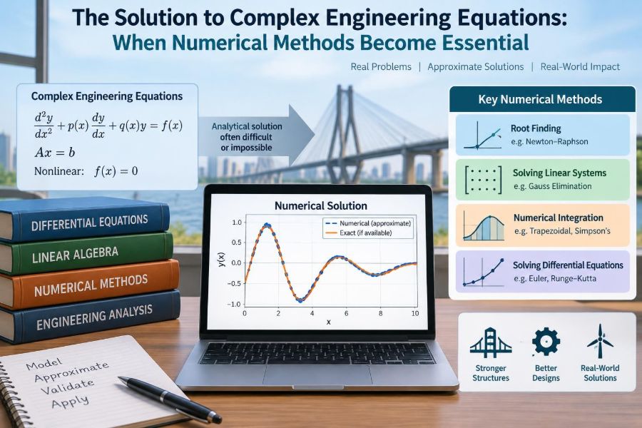

A structural engineer may need to predict how a bridge deck deflects under moving traffic. A chemical engineer may need to calculate temperatures and reaction rates through a reactor. An electrical engineer may be trying to find the operating point of a nonlinear circuit containing diodes.
In each case, the governing equations can be written down from sound physical principles. That is an achievement—but it is not always the end of the problem. The equations may be coupled, nonlinear, time-dependent, or too large to solve exactly with algebra.
This is where numerical methods become part of engineering practice. They replace an impossible or impractical exact calculation with a controlled approximation that can be computed, checked, and improved.
The central skill is not simply pressing “solve” in software. It is knowing what has been approximated, whether the result is believable, and what decision the result can safely support.
🧩 The Point Where Exact Mathematics Stops Helping
An analytical solution is an exact expression, such as a formula for the displacement of a simple beam or the voltage across a basic resistor network. These solutions are elegant, fast to evaluate, and invaluable for understanding fundamental behavior.
Real systems usually add features that break the assumptions required for a tidy formula: irregular geometry, changing material properties, contact between parts, turbulent flow, or loads that vary with time. The governing equations still exist, but an exact closed-form answer may not.
🔢 What a Numerical Method Actually Does
A numerical method converts a continuous mathematical problem into a finite sequence of arithmetic operations. Instead of describing temperature at every point in a metal plate, for example, it estimates temperature at selected locations called nodes.
The method then uses equations to connect those estimates. A computer solves the resulting approximation, producing numbers rather than a single symbolic formula. Those numbers are useful only if the approximation represents the original problem sufficiently well.
🗺️ Continuous Reality, Discrete Models
Engineering physics is often continuous. A pressure field changes across a pipe, stress varies through a component, and a vibrating shaft moves throughout time.
Computers handle finite data. Numerical modeling therefore uses discretization: dividing space, time, or a variable range into manageable pieces. A pipe may be split into short segments; a transient calculation may advance in small time steps.
Discretization is not a flaw to hide. It is a deliberate modeling decision that controls cost, accuracy, and what physical detail the calculation can capture.
📏 Why Real Engineering Equations Become Difficult
Several sources of complexity often appear together. A model might include nonlinear material behavior, a complicated shape, and changing loads at the same time.
- Nonlinearity: doubling an input does not simply double the response.
- Coupling: one field affects another, such as temperature changing structural stress.
- Scale: a discretized model can create thousands or millions of unknowns.
- Uncertain inputs: loads, material data, and boundary conditions may be imperfectly known.
- Time dependence: the present state depends on prior states.
Numerical methods are valuable because they provide practical ways to handle these features, not because they eliminate the need to understand them.
🧠 First Ask Whether a Formula Is Available
Using a numerical method is not automatically the best choice. A simple analytical model can reveal scaling, verify units, expose dominant parameters, and provide a benchmark for a more detailed simulation.
For a simply supported beam under an idealized load, a textbook deflection formula may answer the design question directly. If the same member has openings, variable thickness, contact supports, and a nonlinear material response, a finite element model may be justified.
The effective engineer starts with the simplest model capable of addressing the decision at hand, then adds complexity only when it changes the answer in a meaningful way.
🎯 Defining the Engineering Question Before Solving
A numerical analysis should begin with an output, not a favorite software package. Are you estimating a maximum temperature, locating a resonant frequency, checking a safety margin, or comparing two design options?
The output determines appropriate assumptions and resolution. A model intended to estimate the overall pressure drop in a duct does not need the same level of detail as one intended to investigate local flow separation near a bend.
Clear questions also prevent false precision: reporting many decimal places when the inputs themselves are uncertain.
🧱 Translating Physics into Governing Equations
Numerical work begins with conservation laws and physical relationships. Common examples include conservation of mass, momentum, energy, and electric charge, together with constitutive laws describing how materials respond.
For instance, heat conduction combines energy conservation with a material property called thermal conductivity. Structural analysis combines equilibrium with a stress-strain relationship. The numerical method solves the mathematical model; it cannot compensate for missing physics.
🚪 Boundary Conditions Are Part of the Problem
A differential equation alone rarely defines a unique engineering solution. It also needs boundary conditions, which specify behavior at edges, supports, inlets, outlets, or interfaces.
For a heat-transfer model, a boundary may have a fixed temperature, a prescribed heat flux, or convective cooling to surrounding air. In a structural model, a support may restrain selected motions while permitting others.
Incorrect boundary conditions can yield a calculation that converges perfectly to the wrong physical scenario. This is one of the most common and consequential modeling errors.
📌 Initial Conditions Matter in Transient Problems
When behavior evolves over time, the model also needs an initial condition. A cooling object needs its starting temperature; a dynamic system needs an initial displacement and velocity; a tank model needs an initial fluid level.
An unrealistic starting state can introduce artificial transients. Sometimes those early effects disappear after sufficient simulated time; sometimes they dominate the result. The analyst must decide which is true rather than assuming it.
🔍 Root Finding: Solving One Nonlinear Equation
Many engineering tasks reduce to finding a root: a value of x for which f(x) = 0. Examples include locating the flow rate that balances a pump curve and system resistance, or finding a temperature satisfying an energy balance.
Root-finding methods do not “solve” in one leap. They generate a sequence of guesses that ideally approaches the desired value. Their differences lie in speed, reliability, and the information they require.
✂️ Bisection: Slow, Clear, and Reliable
The bisection method begins with two values that give function values of opposite signs. If the function is continuous between them, a root lies somewhere in that interval. The method repeatedly halves the interval.
It is not the fastest technique, but it is robust when a valid bracket is available. Bisection is especially useful for checking whether a more sophisticated routine is finding a plausible root.
⚡ Newton-Raphson: Fast When the Starting Point Is Good
Newton-Raphson uses the local slope of a function to estimate where its tangent line crosses zero. Near a well-behaved root, it can converge extremely quickly.
Its weakness is sensitivity. A poor initial guess, a nearly flat slope, or a discontinuity can send iterations toward an unintended root or cause divergence. In practice, engineers often combine Newton-type updates with bounds or fallback bracketing methods.
🧮 Systems of Linear Equations Behind Many Models
After discretization, many problems take the form Ax = b. Here, A is a matrix encoding the relationships in the model, x contains unknown values, and b represents loads, sources, or known conditions.
Finite element structural analysis, circuit analysis, and steady heat conduction all commonly produce such systems. The equation may look compact, but the matrix can be enormous for detailed three-dimensional models.
🧷 Direct and Iterative Linear Solvers
Direct methods, such as matrix factorization, seek the solution through a finite sequence of algebraic operations. They can be dependable for modest-sized, well-conditioned systems but may demand substantial memory.
Iterative methods start from an estimate and progressively reduce the residual—the mismatch left in the equations. They are often better suited to very large sparse systems, where most matrix entries are zero.
| Approach | Useful situation | Key caution |
|---|---|---|
| Direct solver | Small to medium systems; repeated confidence checks | Memory and computation can grow rapidly |
| Iterative solver | Large sparse systems | Convergence depends on conditioning and solver settings |
| Preconditioned iterative solver | Difficult large systems | Preconditioner choice affects performance and robustness |
🕸️ Finite Differences: Approximating Change Locally
The finite difference method replaces derivatives with differences between neighboring values. A temperature gradient, for example, is approximated using temperatures at nearby grid points.
It is intuitive and effective for regular geometries such as rectangular plates, straight channels, and simple domains. Its main limitation is handling curved or highly irregular boundaries without elaborate grids.
🔺 Finite Elements: Dividing Complex Shapes into Pieces
The finite element method divides a component or region into small elements connected at nodes. Within each element, the unknown field—such as displacement or temperature—is approximated using simple interpolation functions.
Because elements can follow complicated geometry, finite elements are widely used in structural mechanics, heat transfer, electromagnetics, and many multiphysics applications. Their flexibility is powerful, but it also means mesh design and model setup require judgment.
🌊 Finite Volumes: Conserving What Flows
The finite volume method divides a domain into small control volumes and applies conservation laws to each one. What enters, leaves, is generated, or accumulates must balance within every volume.
This local conservation makes the method especially natural for fluid flow, heat transport, and mass transport. It is commonly associated with computational fluid dynamics, where preserving mass and momentum balances is essential.
⏱️ Time Stepping Turns Motion into a Sequence
Dynamic and transient models advance from one time level to the next. The selected time step determines how much simulated time passes per calculation step.
A very large step may miss rapid changes or become unstable. A very small step can be accurate but expensive. The best choice depends on the physical time scales, the numerical method, and the output that matters.
⚖️ Explicit and Implicit Time Integration
In an explicit scheme, the next state is calculated directly from already known information. These schemes are straightforward and can be efficient per step, but stability may require extremely small time steps.
Implicit schemes solve a coupled set of equations at the new time level. They are often more stable for stiff problems—problems containing processes that evolve on very different time scales—but each step costs more. Stability does not excuse choosing a time step too large to resolve the physics.
🔁 Nonlinear Iteration and Convergence
Nonlinear models are usually solved through repeated updates. At each iteration, the solver evaluates how far the current estimate is from satisfying the equations and adjusts the unknowns.
Convergence means the chosen numerical criteria have been met, often based on residuals or changes between iterations. It does not by itself prove that the model is accurate, physically realistic, or on the correct solution branch.
🚦 Residuals Are Clues, Not Certificates
A residual measures the remaining imbalance in an equation. In a heat model, it can represent the mismatch in energy balance; in a structural model, it can represent unbalanced forces.
Small residuals are generally necessary, but their meaning depends on scaling. A residual that seems numerically small may still be unacceptable relative to the loads or quantities of interest. Always examine both solver diagnostics and physical outputs.
📐 Mesh Resolution and the Cost of Detail
A mesh is the network of elements or cells used to discretize space. Refining it can better capture steep gradients, stress concentrations, thin boundary layers, and curved geometry.
More cells are not automatically better. A dense mesh everywhere wastes resources, while poor-quality elements can harm accuracy even when they are numerous. Refinement should concentrate where the solution changes rapidly or where decisions depend on local behavior.
🔬 Mesh Independence Is a Practical Test
Mesh independence means that a key reported result changes only slightly as the mesh is refined. It does not mean every pointwise value is identical, nor does it require an impossibly fine model.
A practical study compares at least several progressively refined meshes while holding the physical model and solver settings consistent. Track relevant outputs such as peak displacement, pressure loss, or heat-transfer rate—not merely the total number of elements.
🧪 Verification: Did You Solve the Equations Right?
Verification asks whether the numerical implementation correctly solves the mathematical model. Useful checks include comparison with an analytical solution for a simplified case, mesh and time-step studies, conservation checks, and code-to-code comparisons.
For example, before trusting a complex thermal model, an analyst might test the same setup on a one-dimensional wall problem with a known solution. This checks numerical machinery before geometry and added physics obscure the result.
✅ Validation: Are They the Right Equations?
Validation asks whether the model represents the real system well enough for its intended use. It compares predictions with suitable measurements, operational data, or carefully established reference behavior.
A calculation can be verified but not validated: it may solve its equations perfectly while omitting an influential physical effect. Conversely, agreement with a single measurement does not validate a model across all conditions.
📊 Sensitivity Analysis Reveals What Controls the Answer
Every model contains inputs: dimensions, material properties, environmental conditions, source terms, and operating settings. Sensitivity analysis examines how outputs change when these inputs vary within credible ranges.
This process identifies assumptions that deserve better data and those that barely affect the decision. If a design conclusion reverses when a poorly known parameter changes modestly, the result should be treated cautiously rather than presented as settled.
🎲 Uncertainty Is Not the Same as Numerical Error
Numerical error arises from approximation choices such as mesh spacing, time steps, and iteration tolerances. Model uncertainty arises because the physical description is incomplete or simplified. Input uncertainty arises because measurements and future conditions are imperfect.
Improving the mesh reduces only one category. A highly refined simulation cannot make an uncertain load history or unsuitable material law reliable. Good engineering reports distinguish these limitations.
🏗️ Example: A Nonlinear Beam Calculation
Consider a hypothetical slender beam that deflects under an increasing load. At small deflections, a linear beam formula may provide a useful estimate. As deflection grows, the geometry changes enough that the relationship between load and displacement is no longer linear.
A numerical model can apply the load incrementally, update the geometry, and solve equilibrium at each stage. The analysis should check support conditions, material behavior, load increments, convergence, and mesh refinement near regions of high stress.
The result is not simply “the maximum stress.” It is a conditional prediction based on the modeled geometry, loads, constraints, and constitutive assumptions.
🔌 Example: Finding a Circuit Operating Point
A resistor follows a linear voltage-current relation, but a diode does not. A circuit containing both may require the intersection of a nonlinear device characteristic and the rest of the circuit response.
Root finding can determine the operating voltage and current. A plotted curve is often a valuable first check: it can reveal multiple intersections, poor initial guesses, or an input range in which the assumed operating mode is inappropriate.
🌡️ Example: Heat Transfer Through a Complex Part
Suppose an electronic enclosure has heat sources, cooling fins, openings, and materials with different conductivities. Simple resistance-network calculations may estimate overall behavior, but local hot spots depend on geometry and boundary conditions.
A numerical thermal model can estimate the temperature field. Yet its credibility depends strongly on how heat generation, contact resistance, airflow, radiation, and external convection are represented. These inputs may matter more than adding another layer of mesh refinement.
🛑 Common Mistake: Trusting Colorful Contours Too Quickly
Contour plots are persuasive because they turn large datasets into visible patterns. They can also conceal poor setup choices, unsuitable scales, interpolation artifacts, or values outside the physically meaningful range.
Before interpreting a contour, inspect numerical values at critical locations, check conservation balances, review deformation scales, and compare trends with physical expectations. A visually smooth image is not evidence of a correct solution.
🧯 Common Mistake: Treating Solver Failure as a Software Problem
Failure to converge may result from a poor initial guess or unsuitable solver settings. It can also signal a deeper issue: conflicting constraints, missing boundary conditions, unrealistic material data, a physically unstable configuration, or an incorrect equation.
Reducing relaxation factors or increasing iteration limits may help in some cases, but it should not be the first or only response. Inspect the model, residual history, units, and physical plausibility before forcing the calculation onward.
🧰 A Disciplined Workflow for Numerical Problems
- Define the engineering decision and required outputs.
- State assumptions and choose an appropriate physical model.
- Specify geometry, properties, loads, initial conditions, and boundaries.
- Select a method, mesh or grid, time step, and solver strategy.
- Run simple benchmark cases before the full model.
- Check convergence, balances, mesh sensitivity, and time-step sensitivity.
- Validate against relevant evidence when it is available.
- Report results with assumptions, uncertainty, and applicable limits.
This workflow may appear slower than immediately building a detailed simulation. It usually saves time by detecting flawed assumptions before they become polished but unreliable outputs.
💻 Software Automates Arithmetic, Not Engineering Judgment
Modern tools can generate meshes, assemble matrices, run nonlinear solvers, and create sophisticated visualizations. They make problems tractable that would be unreasonable to calculate by hand.
They do not choose the correct physics, recognize a misleading boundary condition, or decide whether a result is fit for a safety-critical decision. Understanding numerical fundamentals makes software more useful because it lets you ask informed questions of every result.
🗣️ Communicating Results So Others Can Trust Them
A useful technical conclusion states more than a final number. It identifies the modeled case, the key assumptions, the numerical checks performed, and the limitations that could materially change the conclusion.
For example: “Under the specified loading and support assumptions, the model predicts a peak displacement within the design criterion; the result was stable under the tested mesh refinements.” That is more informative than presenting a plot without context.
🧭 Choosing the Right Level of Model Fidelity
Model fidelity is the degree of detail included in a simulation. Higher fidelity can capture more mechanisms, but it requires more input data, computing effort, setup time, and opportunities for error.
Early design may need a low-order model that rapidly compares concepts. Final verification may justify a more detailed analysis. The right model is the one that resolves the decision-relevant behavior with evidence proportionate to the consequences of being wrong.
🌟 The Core Principle: Approximate Carefully, Decide Confidently
Numerical methods become essential when engineering equations are too complex for exact formulas, but their purpose is not to replace reasoning with computation. They create a bridge between physical laws and practical predictions.
That bridge is trustworthy when the problem is clearly defined, the assumptions are defensible, the numerical approximation is tested, and the output is interpreted within its limits. A converged answer is only one milestone; a credible engineering conclusion requires the full chain of reasoning.
Numerical methods are most powerful when treated as transparent, testable approximations—not as black boxes that produce unquestionable answers. With that mindset, complex equations become manageable tools for better engineering decisions. 📐💻🔍