
A bridge designer changes the thickness of a steel plate by a few millimetres. An automotive engineer adjusts a cooling channel. A process engineer changes a valve-opening schedule. In each case, the question is deceptively simple: what happens next?
The answer is rarely available as a neat formula. Heat spreads through complicated shapes, fluids swirl and separate, structures bend in many directions, and electrical quantities interact across large networks. Engineering simulation turns those physical questions into calculations a computer can perform.
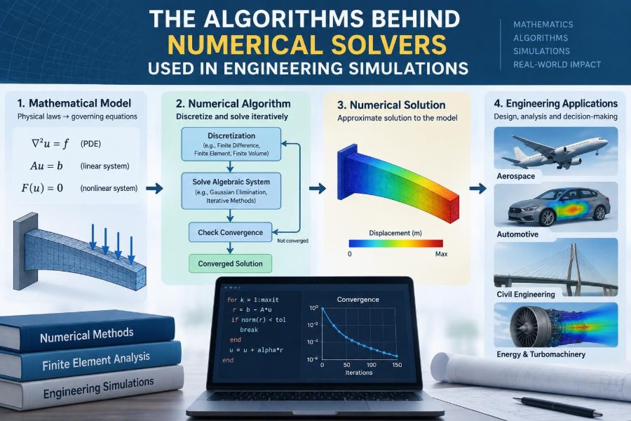
But a simulation result is not produced by a single magic button. Behind the contour plots and animated streamlines are numerical solvers: algorithms that translate equations into a sequence of approximations, tests, corrections, and decisions.
Understanding those algorithms makes simulation software less of a black box. It helps engineers choose appropriate models, recognize misleading results, and spend computation where it actually improves a design.
🧭 What a Numerical Solver Actually Does
A numerical solver is a method for obtaining approximate values from mathematical equations when an exact analytical solution is unavailable or impractical. It takes a model, a geometry, material properties, boundary conditions, and initial conditions, then computes the unknown quantities.
Depending on the problem, those unknowns might be displacement in a bracket, temperature inside a battery cell, pressure in a pipe network, or voltage across a circuit. The solver does not discover the physics; the governing equations and assumptions supplied to it define the physics.
📜 From Conservation Laws to Computable Equations
Most engineering models begin with conservation laws: mass is conserved, momentum changes according to forces, energy is transferred and stored, and electric charge is balanced. These principles lead to differential equations, which describe how a quantity changes with position, time, or both.
For example, heat conduction relates the rate at which temperature changes to the curvature of the temperature field and the material’s thermal properties. Fluid flow uses coupled equations for mass and momentum. The equations may be compact on paper, yet difficult to solve in a real three-dimensional component.
🧩 Why Exact Solutions Usually Run Out
Analytical solutions exist for idealized cases such as steady heat flow through a simple slab or vibration of a uniform beam under carefully chosen conditions. They are invaluable for insight and verification.
Real designs introduce curved geometry, holes, joints, changing materials, nonlinear behavior, moving boundaries, and complex loads. These features usually prevent a closed-form answer. Numerical simulation replaces one hard continuous problem with many smaller algebraic ones.
🕸️ Discretization: Dividing a Continuum into Pieces
Discretization is the central idea. A continuous domain is represented by a finite collection of nodes, cells, elements, or control volumes. Instead of seeking temperature at every conceivable point, the solver calculates it at selected locations and reconstructs the field between them.
A useful analogy is a digital photograph. More pixels can represent sharper detail, but they also require more storage and processing. A computational mesh plays a similar role: it determines where the simulation can resolve variation.
🔺 The Finite Element Method for Structures and Fields
The finite element method, or FEM, divides a body into connected elements such as triangles, quadrilaterals, tetrahedra, or hexahedra. Within each element, the unknown field is represented by simple interpolation functions.
For a structural model, nodal displacements determine the deformation within an element. The element produces a local stiffness relationship, and the software assembles all local relationships into a global system. FEM is also widely used for heat transfer, electromagnetics, acoustics, and coupled problems.
🌊 The Finite Volume Method for Conservation
The finite volume method, or FVM, is common in computational fluid dynamics. It surrounds each computational point with a small control volume and applies conservation directly to that volume.
Fluxes entering and leaving every cell face are balanced with accumulation and sources inside the cell. This makes conservation of mass, momentum, and energy explicit at the discrete level, a major advantage for flow and transport calculations.
📏 Finite Differences on Ordered Grids
The finite difference method approximates derivatives using values at neighboring grid points. A second derivative, for instance, can be estimated from the value at a point and values just to either side.
It is straightforward and efficient on regular rectangular grids. Its limitations become clearer around intricate geometry, where fitting a structured grid to surfaces can be awkward. It remains highly useful in specialized solvers and for building numerical intuition.
🧱 The Mesh Is Part of the Model
A mesh is not merely a visual covering. It controls the discrete equations the solver sees. Elements should be small enough where gradients, stress concentrations, contact zones, boundary layers, or sharp material changes occur.
Refining every location is rarely efficient. A sensible strategy uses finer resolution near a bolt hole or fluid wall and coarser resolution in regions where the solution changes gradually. Poorly shaped elements can also degrade accuracy or slow convergence.
🎯 Shape Functions and Local Approximation
Within an element, a solver needs a rule for estimating values away from nodes. Shape functions provide that rule. Linear elements vary linearly between nodes, while higher-order elements can represent curvature more naturally.
Higher-order elements are not automatically superior. They can capture smooth behavior with fewer elements, but may be more sensitive to distorted geometry, nonlinear contact, or unsuitable integration settings. The right choice depends on the field being represented and the intended accuracy.
🧮 Assembly Creates a Global Linear System
After discretization, many problems take the familiar form Kx = f. Here, K represents the assembled system, x contains unknown values, and f represents applied loads, sources, or boundary contributions.
In linear structural analysis, K is the stiffness matrix and x is displacement. In a thermal problem, the same pattern can represent conductivity and nodal temperatures. Although the notation is compact, the matrix may contain millions of unknowns.
🚪 Boundary Conditions Make the Problem Definite
The equations alone do not specify a unique physical state. Boundary conditions describe what happens at the edges: a fixed support, prescribed temperature, applied pressure, known voltage, insulation, or a fluid inlet and outlet.
Incorrect boundary conditions often produce a polished-looking but meaningless answer. For example, fully fixing a structure that is actually connected through flexible bolts can artificially reduce displacement and change stress paths.
⏱️ Initial Conditions Matter in Transient Analysis
When behavior changes with time, the starting state matters. A transient thermal calculation needs an initial temperature field; a dynamic structural calculation needs initial displacement and velocity; a flow startup may need an initial velocity and pressure field.
A poor initial estimate does not always invalidate the final steady solution, but it can lengthen computation or create nonphysical early behavior. In genuinely transient problems, it directly affects the predicted response.
🔢 Direct Solvers: Reliable but Memory-Hungry
A direct solver transforms a matrix system through systematic factorization, often related to Gaussian elimination. Once factored, it can solve for one or more right-hand sides accurately within numerical precision limits.
Direct methods are attractive for modest-sized systems, difficult conditioning, and cases requiring dependable repeat solutions. Their drawback is memory use and computational cost as the system grows, especially in large three-dimensional models.
🔁 Iterative Solvers: Improving an Estimate Repeatedly
An iterative solver begins with an estimate and repeatedly reduces the residual: the mismatch between the current solution and the discrete equations. Methods such as conjugate gradient and GMRES are designed to reach a useful answer without explicitly factoring the whole matrix.
They can be far more practical for huge sparse systems, where most matrix entries are zero. Yet their performance depends strongly on matrix properties, scaling, and preconditioning. “Iterative” does not mean approximate in a careless sense; it means convergence must be monitored.
🧰 Preconditioning Changes the Difficulty, Not the Physics
A preconditioner is an auxiliary mathematical operation that makes a linear system easier for an iterative method to solve. It aims to improve the matrix’s numerical conditioning while preserving the target solution.
Think of it as reorganizing a difficult route before travelling it. The destination is unchanged, but fewer unproductive turns may be needed. In large simulations, preconditioner selection can matter as much as the iterative algorithm itself.
📉 Residuals Are Not the Same as Error
A small residual means the computed values satisfy the discretized equations closely. It does not prove that the discretized model accurately represents the physical system.
There are at least two separate questions: has the algebraic solver converged, and is the mesh-and-model approximation adequate? A converged answer on a coarse mesh, with unrealistic material data or missing physics, can still be wrong.
🌀 Nonlinearity Turns One Solve into Many
Linear systems assume proportional behavior: double the load, and the response doubles. Many engineering problems violate this assumption. Materials can yield, contact surfaces can open and close, geometry can change under load, and fluid properties can depend on temperature.
Nonlinear solvers address this by solving a sequence of updated linearized problems. Each step uses the latest estimate to revise the equations, then checks whether the solution is sufficiently self-consistent.
📐 Newton’s Method and Tangent Stiffness
Newton-Raphson methods are widely used for nonlinear equations. They use local slope information—often called a tangent matrix or tangent stiffness—to predict a correction to the current solution.
When the initial estimate is reasonable and the problem is well behaved, convergence can be rapid near the solution. But severe contact changes, material softening, or unstable structural behavior can make the iterations struggle, oscillate, or diverge.
🪜 Load Stepping Makes Difficult Changes Manageable
Rather than applying a full nonlinear load in one jump, a solver commonly uses increments. It applies part of the load, converges the response, then proceeds to the next increment.
Small increments often improve robustness because each new state is close to the previous one. They also increase run time. Adaptive schemes adjust increment size: expanding when convergence is easy and cutting back when the solution becomes difficult.
⌛ Time Integration Balances Stability and Cost
Transient simulations replace a continuous time history with discrete time steps. The chosen integration method determines how the solver advances from one time level to the next.
Explicit methods calculate the next state directly from the current one and suit fast wave propagation, impact, and certain highly nonlinear events. Implicit methods solve coupled equations at each step and can take larger steps in many slower processes, such as structural response or heat diffusion.
⚖️ Explicit and Implicit Methods Compared
| Feature | Explicit time integration | Implicit time integration |
|---|---|---|
| Main step cost | Usually lower | Higher because equations are solved each step |
| Stable time step | Often limited by the smallest element and wave speed | Can often be larger, depending on accuracy and nonlinearity |
| Typical uses | Impact, crash, short-duration dynamics | Slow loading, thermal problems, many structural transients |
| Main caution | Tiny stable steps can make runs long | Large steps can miss important dynamics or hinder convergence |
The distinction is practical rather than absolute. The best choice follows the physical time scale, nonlinear behavior, desired outputs, and computational resources.
🌪️ Fluid Solvers Must Couple Pressure and Velocity
In incompressible flow, pressure is not simply evolved like a material property. It acts to enforce mass conservation while velocity is governed by momentum equations. This coupling is a defining challenge in CFD.
Algorithms in the SIMPLE family, pressure-correction approaches, and coupled methods repeatedly update velocity and pressure until the flux balance is acceptable. Under-relaxation may be used to prevent updates from overshooting, particularly in steady nonlinear flow calculations.
🧊 Turbulence Models Add Necessary Assumptions
Turbulent flow contains motion over many length and time scales. Resolving all of them directly is computationally demanding for most engineering geometries, so many simulations use turbulence models to represent unresolved effects.
Reynolds-averaged models, large-eddy simulation, and direct numerical simulation make different accuracy-cost trade-offs. A turbulence model is not a universal correction factor; wall treatment, mesh resolution, flow separation, and calibration assumptions affect whether it is appropriate.
🔗 Multiphysics Means Exchanging Information
Many products involve coupled phenomena: temperature changes material stiffness, flow carries heat, electromagnetic losses generate heating, and deformation alters a fluid passage. A multiphysics solver must transfer information between fields.
Monolithic coupling solves all fields together, which can be robust for strong interactions but computationally demanding. Partitioned coupling alternates between specialized solvers, often conveniently, but may require repeated exchanges to achieve a consistent state.
✅ Verification Asks Whether the Equations Were Solved Right
Verification checks the numerical implementation and solution procedure. Useful practices include mesh refinement studies, time-step refinement, comparison with a simpler benchmark, checking equilibrium, and inspecting residual histories.
A mesh convergence study does not require an unattainably tiny element everywhere. It asks whether the output that drives a decision—peak displacement, pressure drop, heat flux, or fatigue-relevant stress—is becoming insensitive to further refinement.
🔬 Validation Asks Whether the Right Physics Was Solved
Validation compares model predictions with suitable physical observations or experiments. It examines assumptions about material behavior, contact, loads, turbulence, boundary conditions, and other physical inputs.
Verification and validation are complementary. A mathematically correct solution to an oversimplified model is still limited, while a physically thoughtful model cannot compensate for numerical errors or unconverged iterations.
📊 Reading Results Beyond the Color Plot
Color contours are useful, but they can hide choices in scale and interpolation. Always inspect units, extrema locations, deformed-shape magnification, reaction balances, and whether a reported peak occurs at a meaningful physical location.
Singularities deserve particular care. A perfectly sharp re-entrant corner or ideal point load can create stresses that increase without settling as the mesh is refined. The correct engineering response may be to assess stress away from the idealization, revise the local geometry, or use a more suitable failure measure.
⚠️ Common Solver Mistakes and Their Consequences
- Trusting default settings: defaults are starting points, not evidence that the model fits the decision.
- Using one mesh: without refinement evidence, a reported peak may be a mesh artifact.
- Chasing residuals alone: low residuals cannot repair missing loads or unrealistic constraints.
- Taking oversized time steps: a stable calculation can still smooth out important transient behavior.
- Ignoring solver warnings: convergence difficulties often reveal physical discontinuities, poor constraints, or unsuitable controls.
🛠️ A Practical Workflow for Robust Simulations
- State the engineering question and the output that will support a decision.
- Choose governing physics and simplify only with a stated rationale.
- Apply loads, constraints, properties, and initial conditions with checks for units and realism.
- Build a mesh targeted at expected gradients and critical regions.
- Select solver controls appropriate to linearity, time scale, and coupling strength.
- Check convergence, conservation, refinement sensitivity, and physical plausibility.
- Document assumptions and uncertainty alongside the final result.
This workflow is deliberately iterative. A surprising result should prompt inspection of the model, not immediate adjustment until the plot looks familiar.
🧠 Choosing a Solver Starts with the Question
There is no universally best algorithm. A static elastic bracket may be handled efficiently by a linear FEM solve; a crash event may require explicit dynamics; an internal flow problem may favor finite volumes and pressure-velocity coupling; a slowly heated assembly may need nonlinear transient analysis.
The core choice is driven by the relevant physics, geometry, output quantity, accuracy requirement, and available computational budget. Software labels matter less than understanding what equations and assumptions the selected workflow actually uses.
🏁 The Core Principle Behind Trustworthy Results
Numerical solvers are disciplined approximation machines. They discretize physical laws, solve large systems of equations, manage nonlinearity and time evolution, and report whether their internal algebraic targets have been met.
Trust emerges when three layers agree: the physical model is appropriate, the numerical approximation is sufficiently resolved, and the solver has converged. None of those layers can substitute for the others.
A simulation earns confidence not because it produces a detailed image, but because its assumptions, algorithms, and checks support the engineering decision being made. That is the practical mathematics behind every useful solver run. 📐⚙️