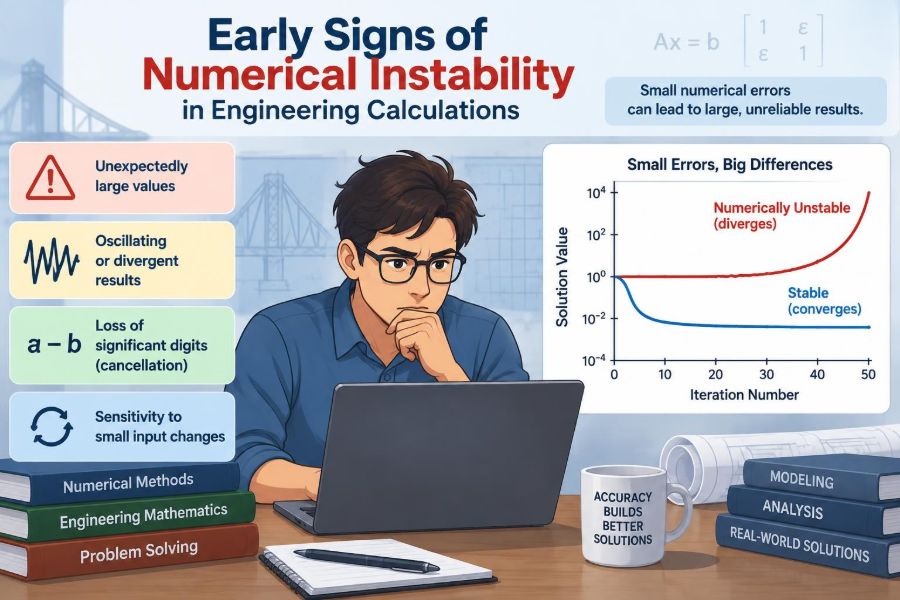

A simulation that ran smoothly yesterday can suddenly produce a pressure spike, a negative concentration, or a displacement so large that the plotted curve vanishes off the screen. The model may look correct. The code may contain no obvious error. Yet the result is no longer describing the physical system.
This is a familiar engineering problem because numerical calculations are not exact algebra. Computers represent numbers with limited precision, approximate derivatives and integrals, and solve large systems through finite sequences of operations. Small numerical defects can be harmless—or they can be amplified at every step.
The most useful time to detect instability is before a solver crashes or a design decision is made from unreliable output. Early warning signs often appear in residuals, step histories, mesh refinements, or values that merely look a little odd.
Learning to recognise those signs turns numerical stability from a mysterious software issue into an engineering habit: observe, question, test, and only then trust the result.
🔎 What numerical instability actually means
Numerical instability occurs when unavoidable computational errors grow rather than remain controlled. Those errors may come from rounding, approximate equations, incomplete convergence, noisy input data, or an unsuitable algorithm.
It is not the same as a physical instability. A bridge model can report wildly oscillating displacements even if the physical structure is stable; conversely, a physical buckling or vibration instability can be represented accurately by a numerically stable calculation. The key question is whether changes in the computed result are caused by the modeled physics or by the calculation method.
🧭 Why early detection matters in engineering
An unstable calculation can waste more than computing time. It can hide a modeling mistake, lead to an overdesigned component, or create false confidence in a marginal design. In control, thermal, fluid, and structural problems, unstable numerical output can also obscure the operating conditions that truly matter.
Early diagnosis is usually cheaper than post-processing a failed model. A changing residual pattern or a solution that depends heavily on time step may reveal the issue while the model is still small and understandable.
🧮 The small errors behind large failures
Most engineering calculations use floating-point arithmetic: numbers are stored with a finite number of binary digits. Values such as 0.1 generally cannot be represented exactly, so each operation introduces a tiny rounding difference.
One small difference is rarely concerning. Trouble begins when an algorithm repeatedly magnifies it, such as by subtracting nearly equal numbers, differentiating noisy data, or taking thousands of time steps in a sensitive system. Stability describes whether that amplification remains bounded.
📉 A solution that changes when precision changes
A practical early sign is excessive sensitivity to arithmetic precision. If a calculation gives materially different engineering conclusions in single precision and double precision, investigate before deciding which answer is “right.”
Different digits at the far end of a long decimal are expected. Different peak stresses, convergence behaviour, or safety margins are not. Precision comparisons are especially revealing when the model contains large differences in scale, such as micrometre displacements alongside kilometre coordinates.
🌊 Oscillations that should not be there
Unexpected alternating values are one of the clearest warning signs. A temperature at a node may jump above and below its neighbours, or a nonlinear iteration may overshoot from one side of a solution to the other without settling.
Some oscillation is physically valid: vibrating machinery, pressure waves, and switching circuits naturally oscillate. Suspicion is warranted when the frequency follows the numerical grid or iteration count rather than a known physical timescale, or when refining the grid changes the pattern dramatically.
⏱️ Time-step sensitivity in transient models
In transient analysis, repeat a representative case with smaller time steps. If the solution changes substantially as the step is reduced, the original step was not resolving the process adequately—or the time-integration scheme may be unstable for that step size.
For example, an explicit heat-transfer calculation can become unstable when the time step is too large relative to material diffusivity and element spacing. Temperatures may then alternate unrealistically between high and low values instead of diffusing smoothly.
🕸️ Mesh dependence is a diagnostic clue
Finite element and finite volume models replace a continuous domain with a mesh. A finer mesh can reveal more local detail, so some change is normal. But global outputs should generally approach a stable trend as the mesh is refined.
If stress peaks, pressure drops, or natural frequencies drift continually with no sign of convergence, do not simply select the finest affordable mesh. The issue may be an unresolved singularity, poor element quality, inadequate boundary conditions, or a formulation that needs a different treatment.
📏 Distinguish convergence from correctness
A solver reporting “converged” means it met its internal stopping criteria. It does not prove that the equations, material model, constraints, mesh, and units represent the real problem correctly.
Likewise, a non-converged solve is not automatically useless. It may be close to a meaningful state, or it may be following an invalid path. Treat convergence as evidence about the numerical process, then verify the engineering result independently.
🎯 Residuals that stall, rise, or zigzag
A residual measures how far the current numerical estimate is from satisfying the governing equations. In an iterative solve, residuals commonly decrease as the estimate improves.
Watch for residual histories that flatten far above the tolerance, rise after an initially promising decrease, or zigzag indefinitely. These patterns can indicate a poorly conditioned matrix, an unsuitable iteration method, excessive nonlinear loading, or conflicting constraints. A single final residual value reveals much less than the complete history.
🔁 Iterations that need constant rescue
Many nonlinear solvers use damping, relaxation, line searches, or automatic step reductions to recover from difficult iterations. These are useful tools, not proof of failure.
However, a solve that only succeeds after repeated emergency reductions is sending a message. The model may contain a sharp contact transition, an abrupt material law, a bad initial estimate, or a load increment too large for the nonlinear path. Record how often these controls activate rather than judging only whether the run eventually finishes.
⚖️ Ill-conditioning and nearly dependent equations
A system is ill-conditioned when small changes in input produce disproportionately large changes in the calculated solution. This often arises when equations are nearly redundant, material properties differ by many orders of magnitude, or a structure has a nearly free rigid-body motion.
Ill-conditioning does not always cause an error message. It may show up as slow convergence, wildly varying reactions, or a solution that changes after harmless-looking edits. Matrix condition estimates, pivot warnings, and sensitivity checks are valuable clues when the software exposes them.
🧷 Near-zero pivots and singular matrices
A singular matrix cannot be uniquely solved. In structural analysis, a common cause is missing restraint: the model can translate or rotate as a rigid body. In circuit analysis, it may be a floating node with no defined reference.
A near-singular matrix is more subtle. The model technically has a solution, but it is so weakly constrained that round-off can dominate part of the answer. Do not silence these warnings by adding arbitrary restraints or tiny springs without documenting their physical meaning and checking their influence.
📐 Bad scaling makes healthy models look sick
Numerical algorithms work best when variables and equations have broadly comparable magnitudes. Mixing forces in newtons, stiffnesses in gigapascals, coordinates in millimetres, and tolerances in dimensionless defaults can make meaningful changes invisible to a solver.
Scale variables where possible, use consistent units, and select tolerances related to the problem’s physical size. A displacement tolerance suitable for a metre-scale mechanism may be inappropriate for a micromachined device.
➖ Catastrophic cancellation in subtraction
Catastrophic cancellation happens when two nearly equal numbers are subtracted. Their leading digits cancel, leaving a result whose useful precision can be very poor.
Consider estimating a small difference between two large energies or pressures. Each quantity may be computed with a minor relative error, yet their difference can have a large relative error. Reformulating an expression analytically, rescaling variables, or using a numerically stable library function can avoid this trap.
🧊 Tiny values, overflow, and underflow
Overflow occurs when a computed value is too large to store; underflow occurs when it is so small that the computer rounds it toward zero. Both can quietly corrupt later calculations before producing an obvious infinity or “not a number” result.
Exponential models, high powers, likelihood-like products, and repeated matrix operations are common locations. Inspect intermediate ranges, use logarithmic forms when mathematically appropriate, and add checks for non-finite values immediately after critical operations.
🧱 Discontinuities that confuse smooth solvers
Many efficient numerical methods assume that a function changes smoothly. A model with abrupt contact, switching controls, piecewise material properties, or on-off logic can violate that assumption.
The result may be iteration chatter near a threshold: one iteration activates contact, the next deactivates it, and the process repeats. The physical discontinuity may be real, but it often requires a solver designed for nonsmooth behaviour, smaller increments, or carefully justified regularisation.
🧨 Unstable explicit integration
Explicit time-integration schemes calculate a new state directly from previously known states. They are attractive for fast, highly nonlinear events, but they commonly have a critical time step set by the smallest elements and fastest wave speeds in the model.
When that limit is exceeded, numerical energy can grow rapidly. A practical sign is a response that becomes increasingly noisy, energetic, or distorted without a plausible source of external energy. Reducing the time step is a direct test, but changes to mesh and material assumptions should also be reviewed.
🧩 Implicit solvers have different failure modes
Implicit methods are often more tolerant of large time steps for certain problems, but “unconditionally stable” claims must be interpreted carefully. Stability of a linearized integration scheme does not guarantee accuracy, nonlinear convergence, or faithful treatment of rapid events.
An implicit dynamic model can damp real high-frequency motion if its time step is too large. It may look calm and stable while missing the physics. Numerical stability and temporal resolution must be checked separately.
📈 Energy balance as a physical audit
Energy is a powerful cross-check in mechanics. Depending on the problem, compare external work with kinetic energy, strain energy, internal dissipation, and constraint or contact contributions.
Some methods introduce controlled numerical damping or artificial energy terms, so exact equality is not always expected. But unexplained growth, a dominant artificial contribution, or an energy jump that does not match loading deserves investigation. The same principle applies in thermal and fluid models through mass, heat, and momentum balances.
🧪 Conservation errors reveal hidden trouble
For a closed system, mass should not appear or disappear without a modeled mechanism. In a flow calculation, monitor net mass flux; in a heat model, compare stored energy with heat entering and leaving; in an electrical network, check current balance at nodes.
Small discrepancies can arise from tolerances and discretisation. A growing imbalance over time, however, is often an early indicator of unstable updates, inconsistent boundary conditions, or an implementation error in a custom calculation.
🧷 Boundary conditions can create numerical symptoms
Unrealistic boundary conditions are sometimes mistaken for numerical instability because they produce extreme gradients and concentrated reactions. Fixing a component too rigidly, applying a point load where a distributed load belongs, or prescribing incompatible displacements can make a model exceptionally hard to solve.
Before changing solver settings, sketch the physical load path. Ask what prevents each motion, where forces enter, and whether the idealisation introduces singular behaviour. A numerically robust model still needs physically defensible constraints.
🔬 Verify with a simpler version first
A reduced model is often the fastest troubleshooting tool. Remove secondary features, use linear material behaviour, simplify geometry, or solve a one-dimensional analogue with a hand calculation.
If the simplified case behaves sensibly, reintroduce features one at a time. If it fails too, the issue is likely foundational: units, signs, boundary conditions, governing equations, or solver setup. This controlled approach is usually more informative than changing many settings at once.
🧾 Use independent checks, not repeated runs
Running the same model repeatedly confirms only that it is repeatable under the same assumptions. Verification is stronger when it uses an independent route: a limiting-case formula, an alternative discretisation, a second solver, a conservation law, or a deliberately coarse hand estimate.
For example, a cantilever model should recover the expected qualitative relation between load, length, stiffness, and deflection. The comparison need not be exact to reveal a reversed load direction, an incorrect section property, or a unit conversion error.
🗂️ Monitor the right quantities during a solve
Do not wait for a colourful final contour plot. Track a small set of diagnostic quantities throughout the calculation:
- residual norms and iteration counts;
- time-step or load-increment changes;
- maximum and minimum state variables;
- mass, energy, charge, or other conserved balances;
- contact status, constraint reactions, or active-set changes;
- non-finite values, warnings, and solver restarts.
These records make a failure explainable. They also help distinguish a difficult but valid physical transition from a calculation that is losing control.
🛠️ A disciplined response when warning signs appear
When results look suspicious, resist the urge to immediately tighten every tolerance or switch to a more expensive solver. First identify whether the symptom is temporal, spatial, algebraic, nonlinear, or physical.
- Save the case and record the first abnormal step.
- Check units, signs, constraints, and input ranges.
- Plot residuals and key balances, not just final fields.
- Repeat with a smaller time step or refined mesh.
- Compare with a simplified or independently checked case.
- Change one numerical control at a time and document the effect.
This sequence builds evidence instead of producing a collection of unexplained parameter changes.
🚫 Common fixes that only hide the issue
Several common responses can make a run finish while making the answer less trustworthy. Adding artificial damping may suppress oscillations but also erase real dynamics. Relaxing convergence tolerances may accept an inaccurate equilibrium. Limiting output ranges can conceal growing values without correcting them.
Likewise, adding weak springs, numerical viscosity, or smoothing parameters can be legitimate modelling choices when physically justified and sensitivity-tested. They become risky when used solely to remove warnings. Every stabilising device should have a stated purpose and a measurable influence on the quantities that matter.
🧑💻 Practical habits for spreadsheets and scripts
Numerical instability is not limited to advanced simulation software. Spreadsheets can propagate a wrong reference through thousands of cells, while scripts can silently reuse stale arrays or divide by nearly zero quantities.
Build simple safeguards: assert expected ranges, flag missing or non-finite data, print intermediate norms, and test functions with known inputs. Keep calculations modular so a derivative, matrix assembly, or interpolation routine can be tested in isolation.
📊 A compact warning-sign reference
| Observed sign | Possible numerical cause | Useful first check |
|---|---|---|
| Alternating node values | Time-step instability or poor discretisation | Reduce time step and inspect mesh pattern |
| Residuals stop decreasing | Ill-conditioning or nonlinear path difficulty | Review constraints, scaling, and increment size |
| Results move with mesh refinement | Unresolved gradient or singularity | Perform a structured mesh-convergence study |
| Huge values after a few steps | Overflow, unstable update, or unit error | Inspect intermediate magnitudes and units |
| Different answers after small edits | Near-singularity or poor conditioning | Check supports, matrix diagnostics, and scaling |
🧠 Build confidence gradually, not all at once
Trust in a numerical result should increase through layers of evidence. Start with correct dimensions and sensible limiting behaviour. Then check convergence in time, space, and iteration. Finally compare with measurements, established benchmarks, or another credible model when those are available.
No single test proves correctness. A mesh-converged answer can still use the wrong boundary condition, and a converged nonlinear solve can still rely on implausible material data. Confidence comes from independent checks that fail in different ways.
✅ The core principle: investigate amplification
The early signs of numerical instability are rarely mysterious once you know where to look: unexplained oscillations, sensitivity to step size or mesh, stalled residuals, conservation drift, impossible values, and extreme dependence on small changes.
Each sign points to the same underlying question: is the calculation controlling small errors, or is it amplifying them? Answering that question requires numerical diagnostics and engineering judgement together. Neither solver messages nor attractive plots can replace that combination.
Reliable engineering calculations are built by testing whether results remain stable when the numerical path is challenged, not by accepting the first run that completes. That habit protects both the model and the decisions made from it. 📐🔍⚙️