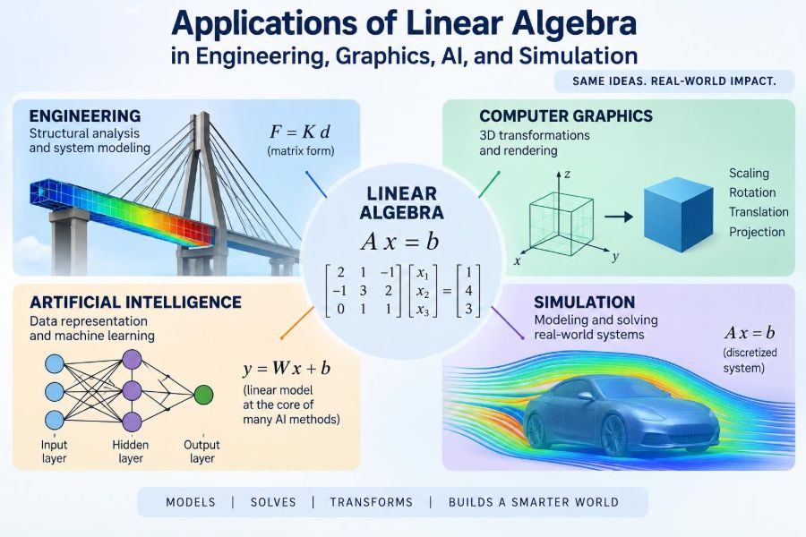

A navigation app redraws a route as traffic changes. A phone recognizes a face in a photo. A bridge model predicts how a structure will bend under load. A game rotates a virtual camera through a detailed 3D world without the scene falling apart.
These tasks look unrelated, but many rely on the same mathematical language: vectors, matrices, and transformations. This is linear algebra—a subject that can initially feel abstract because its symbols are compact while its uses are everywhere.
For engineers, linear algebra turns large systems of relationships into forms that computers can store and solve. For graphics and simulation, it describes position, motion, light, and shape. For artificial intelligence, it provides the machinery for learning patterns from large collections of numbers.
The goal is not merely to manipulate matrices by hand. It is to recognize what a matrix represents, choose an appropriate model, and understand when a numerical answer deserves trust.
🧭 Linear Algebra as a Language of Relationships
Linear algebra studies quantities that combine in predictable ways. A vector usually represents several related values: a force with horizontal and vertical components, a sensor reading with many channels, or the coordinates of a point.
A matrix is a rectangular arrangement of numbers that describes a relationship between vectors. It can transform an input into an output, such as converting actuator commands into motion or pixel values into a changed image.
This viewpoint matters because engineering problems rarely contain one isolated variable. They involve many variables that influence one another at once.
➡️ Vectors Describe Direction, State, and Data
In geometry, a vector has magnitude and direction. A two-dimensional velocity vector, for example, records both how fast an object moves and where it is headed.
In engineering, “vector” has a broader practical meaning: an ordered list of numbers. The state of a small drone might include position, velocity, orientation, and angular velocity. Putting these values in one vector makes them easier to update, compare, and use in equations.
The order and units matter. Combining a displacement measured in metres with a temperature measured in degrees may be mathematically possible, but it only becomes meaningful when the model explains why those quantities belong together.
🔢 Matrices Encode Systems Efficiently
A matrix can be read as a compact rule. In the expression Ax = b, the matrix A contains the system relationships, x is the unknown vector, and b is the known outcome or input.
For a circuit, the entries of A may come from resistances and connection rules. For a truss, they can represent how member forces contribute to balance at each joint. One matrix may capture hundreds or millions of coupled equations.
Rows often correspond to equations or observations; columns often correspond to unknowns or features. That interpretation is more useful than seeing a matrix as a grid to be memorized.
🧮 Matrix Multiplication Represents Composition
Matrix multiplication is not ordinary element-by-element multiplication. It combines relationships. If one matrix converts a local coordinate into a robot-arm coordinate and another converts that coordinate into a world coordinate, multiplying them creates one direct local-to-world transformation.
Order is crucial. In general, AB is not equal to BA. Rotating an object and then translating it usually gives a different result from translating it and then rotating it.
This is a frequent source of graphics and robotics bugs. The arithmetic may be correct while the transformations are applied in the wrong sequence.
📐 Coordinate Systems Make Geometry Usable
Every engineering model needs a frame of reference. A vehicle may have a body-fixed coordinate system, a map-based world system, and a camera system, each with different origins and axes.
Linear algebra converts coordinates between these frames. A point that is “two metres ahead” of a vehicle is simple in the vehicle frame, but its location on a map depends on the vehicle’s current position and heading.
Clear frame naming prevents confusion. In professional work, a transformation should state what it converts from and to, rather than being labelled only as a vague “rotation matrix.”
🔄 Transformations: Scaling, Rotation, and Shear
A linear transformation changes vectors while preserving straight-line structure and the origin. Common examples include scaling, rotation, reflection, and shear.
Scaling changes size along one or more axes. Rotation changes direction without changing distance from the origin. A shear slants an object by shifting one coordinate in proportion to another; it appears in geometric modelling and some deformation calculations.
These operations can be represented by matrices, allowing a computer to apply the same geometric rule to many points rapidly and consistently.
🏗️ Homogeneous Coordinates Add Translation
Translation—moving an object without rotating or resizing it—is not linear in ordinary Cartesian coordinates because it does not keep the origin fixed. Graphics and robotics solve this neatly with homogeneous coordinates.
A 3D point (x, y, z) is represented with an additional coordinate, commonly as (x, y, z, 1). A 4×4 matrix can then represent rotation, scale, and translation together.
This convention makes transformation pipelines easier to combine. It also explains why 4×4 matrices are so common in 3D software even when the scene itself is three-dimensional.
🎮 The Graphics Transformation Pipeline
Rendering a 3D scene requires several coordinate changes. A model begins in its own local coordinates, is placed in the world, viewed from a camera, and projected onto a two-dimensional screen.
- Model transformation: positions the object in a scene.
- View transformation: expresses the scene relative to the camera.
- Projection transformation: creates perspective or an orthographic view.
- Viewport transformation: maps the result to screen pixels.
Each step is matrix-based. Keeping the stages separate makes it easier to diagnose a model that appears mirrored, clipped, or unexpectedly far away.
👁️ Projection Turns 3D Scenes into Images
Perspective projection makes distant objects appear smaller, resembling human visual experience and camera images. Orthographic projection keeps parallel lines parallel and does not make objects shrink with distance.
Neither is universally better. Perspective is useful for realistic visualization and games; orthographic views are valuable in CAD, technical drawing, and measurement-focused interfaces because scale is more visually consistent.
Projection also has limits. Objects outside the viewing region are clipped, and points behind a camera require careful handling. These are geometric consequences, not simply display errors.
🌈 Images Are Matrices Too
A grayscale digital image can be represented as a matrix whose entries are pixel intensities. A colour image usually contains several such arrays, commonly one for each colour channel.
This representation enables operations such as blurring, sharpening, edge detection, resizing, and geometric warping. A filter examines nearby pixels using a small array of weights, often called a kernel.
Image processing is not only visual. Similar methods help inspect manufactured surfaces, track objects in video, read documents, and prepare data for machine-learning systems.
🧱 Finite Element Analysis Breaks Structures into Parts
Finite element analysis, or FEA, models a complex part by dividing it into many small connected elements. Within each element, displacement or temperature is approximated using relatively simple functions.
The local behavior of each element becomes a small matrix. Assembly combines these contributions into a larger system describing the full structure, machine component, or thermal field.
A solver can then estimate quantities such as deflection, stress, vibration modes, or heat flow. The method is powerful, but its result remains a model: mesh quality, material assumptions, loading conditions, and boundary constraints all affect reliability.
⚖️ Stiffness Matrices Connect Force and Deflection
In a basic structural model, the equation K u = f is central. Here, K is the stiffness matrix, u contains unknown displacements, and f contains applied forces.
The matrix records how movement at one degree of freedom affects forces at others. A force applied near one point of a frame can therefore influence displacement throughout the structure.
Boundary conditions are essential. If supports are omitted or incorrectly specified, the system may have no unique solution—or produce movement that is physically impossible.
🌡️ Heat, Fluids, and Field Problems
Many physical processes are described by fields: temperature at every point in a component, pressure throughout a pipe network, or electric potential across a device. Discretization replaces the continuous field with values at selected nodes or cells.
The resulting equations are often large and sparse, meaning most matrix entries are zero because each location interacts mainly with nearby locations. Sparse storage and algorithms make these models computationally practical.
Fluid simulations add difficulty because velocity, pressure, turbulence models, and moving boundaries can interact strongly. Linear algebra remains fundamental, but the full problem may require repeated solution of changing linearized systems.
⚡ Electrical Networks Become Linear Systems
Kirchhoff’s current and voltage laws lead naturally to matrix equations. In nodal analysis, unknown node voltages form a vector, while conductances and circuit connections populate a matrix.
For linear resistive circuits, the result can be solved directly. Capacitors, inductors, nonlinear components, and time-varying sources require additional modelling, but each simulation step commonly still involves linear algebra.
This method scales far better than manually writing separate equations for each branch. It also makes it easier for circuit-design tools to analyze many operating conditions.
🤖 Robotics Uses Matrices for Pose and Motion
A robot’s pose combines position and orientation. Homogeneous transformation matrices describe the pose of each arm link, sensor, or tool relative to another frame.
Forward kinematics calculates where an end effector will be from known joint angles. Inverse kinematics works backward: it seeks joint values that place a tool at a desired location and orientation.
Inverse kinematics may have several solutions, no feasible solution, or configurations that are sensitive to small changes. Joint limits, collisions, and actuator constraints must therefore be considered alongside the matrix equations.
📡 State-Space Models Guide Control Systems
Control engineering often expresses dynamic behavior in state-space form: ẋ = Ax + Bu and y = Cx + Du. The state vector x stores information needed to predict future behavior, such as position and velocity.
The matrices define internal dynamics, control inputs, measurements, and direct feedthrough. This formulation works naturally for systems with several inputs and outputs, from aircraft motion to motor drives.
A linear state-space model is often an approximation around a chosen operating point. It can be highly useful near that condition but may not capture saturation, friction, backlash, or large nonlinear motions without extensions.
📈 Eigenvalues Reveal Characteristic Behavior
An eigenvector is a direction that a transformation changes only by scaling. Its associated eigenvalue gives that scaling factor. This idea helps identify natural modes of behavior in many systems.
In vibration analysis, mode shapes describe characteristic deformation patterns, while related eigenvalues connect to natural frequencies under a model’s assumptions. In control, eigenvalues of a system matrix help assess whether small disturbances tend to decay or grow.
Eigenvalues are diagnostic tools, not automatic safety certificates. A physical system can behave differently when unmodelled effects, nonlinearities, or changing operating conditions become significant.
🎵 Singular Value Decomposition Finds Structure
Singular value decomposition, or SVD, factors a matrix into rotations or reflections plus directional scaling. Unlike some eigenvalue methods, it applies broadly to rectangular matrices, including data tables with different numbers of rows and columns.
The largest singular values identify directions in which the data or transformation has the greatest effect. Small singular values can reveal directions that are weakly determined or highly sensitive to noise.
SVD supports image compression, recommendation systems, signal processing, and stable numerical methods. It is computationally demanding for very large dense matrices, so practical implementations often use approximations or exploit structure.
🗜️ Low-Rank Approximation Compresses Information
Many data sets contain redundancy. A low-rank approximation keeps only the dominant patterns in a matrix rather than every detail.
For example, a hypothetical photograph may be approximated by retaining its strongest SVD components. The file can become smaller, but fine texture and sharp edges may be lost if too few components remain.
The trade-off is central: reducing rank can suppress noise and storage cost, yet it may discard subtle but meaningful information. In engineering data, that lost detail might include a small defect signal rather than random variation.
🧠 Machine Learning Runs on Vectors and Matrices
Machine-learning models convert inputs into numerical feature vectors. A row might represent one product, image, sensor window, or customer interaction; columns represent measured or derived features.
Neural networks repeatedly apply matrix multiplications, add bias vectors, and use nonlinear activation functions. Training adjusts the matrix entries—often called weights—so outputs better match examples according to a chosen loss function.
Linear algebra makes these operations efficient on modern hardware. It does not make a model automatically valid: biased data, poor labels, leakage between training and evaluation data, and weak problem definitions can still produce misleading systems.
🔍 Principal Component Analysis Simplifies Features
Principal component analysis, or PCA, finds orthogonal directions that capture substantial variation in a data set. It can reduce many correlated measurements to fewer transformed variables called principal components.
For a sensor-rich machine, PCA may help visualize operating patterns or reduce input size before another analysis. The components are combinations of original variables, so they may be less intuitive than directly measured quantities.
Variance is not the same as importance. A low-variance feature can still matter for fault detection or safety, which is why PCA should be selected based on the task rather than treated as a universal preprocessing step.
🎯 Least Squares Handles Imperfect Measurements
Real measurements rarely satisfy every equation exactly. Least squares finds a solution that minimizes the sum of squared residuals—the differences between observed values and model predictions.
It is used in curve fitting, camera calibration, GPS-style positioning, parameter estimation, and sensor fusion. When data contain occasional large outliers, ordinary least squares can be overly influenced by them.
Robust estimation, measurement screening, and uncertainty analysis may be more appropriate in such cases. A small residual alone does not prove that the underlying model is physically correct.
🧭 Optimization Links Decisions to Constraints
Linear algebra is closely connected to optimization. Many design and scheduling problems ask for a vector of decisions that minimizes cost, weight, energy, or error while satisfying constraints.
In linear programming, both objectives and constraints are linear. More advanced optimization may include quadratic terms, integer decisions, nonlinear models, or uncertainty, but matrices still organize the constraints and derivatives.
For example, a production plan can be represented by a decision vector, while material availability and machine capacity become matrix constraints. The solution is only as useful as the assumptions about demand, capacity, and priorities.
🧪 Simulation Advances Systems in Time
Simulations often update a state vector from one time step to the next. For a simple discrete linear model, this can look like x(k+1) = A x(k) + B u(k).
This pattern appears in sampled control systems, population-like flow models, simplified thermal models, and animation. More detailed physical simulations may solve a new matrix equation at every time step.
Time-step size matters. Steps that are too large can miss rapid behavior or create numerical instability; steps that are very small can be expensive. Choosing a method requires balancing accuracy, stability, and available computing time.
🧩 Sparse Matrices Make Large Models Feasible
Large engineering matrices are frequently sparse. In a finite element mesh, a node affects nearby nodes, not every node in the model. Storing all the zeros would waste memory and processing effort.
Sparse matrix formats record only nonzero entries and their locations. Specialized solvers then exploit that structure, allowing much larger systems to be handled than dense methods would permit.
Reordering variables can also reduce computational work by limiting “fill-in,” where zeros become nonzeros during factorization. Such implementation details can determine whether an analysis runs in a useful time or not.
💻 Direct and Iterative Solvers Have Different Roles
Direct methods, such as matrix factorization, aim to solve a system in a finite sequence of operations under ideal arithmetic. They are often reliable for moderate-sized, well-structured problems and can be convenient when many right-hand sides share one matrix.
Iterative methods improve an approximate solution over repeated steps. They can be highly effective for enormous sparse systems, but convergence depends on matrix properties, stopping criteria, and often a preconditioner that improves numerical behavior.
The right choice depends on problem size, sparsity, conditioning, required accuracy, and computing resources—not on a single solver being universally superior.
⚠️ Conditioning Determines Sensitivity to Error
A system is poorly conditioned when small changes in input data can create large changes in the solution. This can occur when equations are nearly redundant or when a matrix is close to singular.
Measurement noise, rounding, and limited numerical precision then become more consequential. A computed answer may look precise on screen while being physically uncertain.
Useful responses include rescaling variables, revisiting the model, collecting better measurements, regularizing an underdetermined problem, or reporting uncertainty instead of presenting excessive decimal places.
📏 Units, Scaling, and Nondimensionalization
Matrices often mix variables with different units and magnitudes. A model involving millimetres, megapascals, milliseconds, and kilowatts can be difficult to interpret and numerically awkward if values vary across many orders of magnitude.
Consistent units are the first safeguard. Scaling variables so typical values are closer in magnitude can improve conditioning and make solver tolerances more meaningful.
Nondimensionalization goes further by expressing variables relative to characteristic reference values. It can reveal which effects dominate a system and help compare designs operating at different physical scales.
🛠️ A Practical Workflow for Matrix-Based Problems
A dependable workflow starts before any solver is called. Define the physical question, identify the relevant variables, and decide which relationships can reasonably be approximated as linear.
- State the input, output, units, assumptions, and coordinate frames.
- Build the vector and matrix representation from governing laws or data.
- Check dimensions, signs, boundary conditions, and limiting cases.
- Select a solver suited to the matrix structure and accuracy needed.
- Validate results against physical intuition, measurements, or simpler cases.
- Document uncertainty, parameter choices, and conditions under which the result applies.
This process catches more errors than focusing only on algebraic manipulation.
🚫 Common Mistakes in Applied Linear Algebra
One common mistake is treating a matrix as detached from the system it represents. This makes sign errors, transposed dimensions, and incorrect variable ordering much harder to notice.
Other recurring problems include:
- using coordinate transformations in the wrong order;
- confusing row vectors with column vectors in software conventions;
- inverting a matrix explicitly when a solver would be more stable and efficient;
- ignoring singularity or poor conditioning warnings;
- trusting a plausible visualization without checking units and constraints.
Good notation, small test cases, and independent checks are practical defenses against these failures.
🔗 The Core Principle: Structure Makes Complexity Manageable
Linear algebra succeeds because it exposes structure. Vectors collect related quantities, matrices encode relationships, and decompositions reveal dominant directions, modes, or hidden redundancy.
That structure connects a rotating game object, a flexible beam, a camera image, a feedback controller, and a trained AI model. Their applications differ, yet each gains from representing many interacting quantities in an organized mathematical form.
The deepest practical lesson is to connect every operation back to meaning: what does this vector describe, what transformation does this matrix perform, and what assumptions make the result credible?
Linear algebra is most valuable when it turns a complex real system into a model that is both computable and understandable. Learn the interpretation alongside the calculation, and matrices become tools for reasoning—not just arrays of numbers. 📐🤖⚙️