
A pump is operating in a process plant, and its vibration signal begins to drift. The maintenance team has historical sensor records, but only a few examples of failures. A purely data-driven model may spot patterns, yet it can also make confident predictions that violate basic mechanics.
Now consider a bridge, a battery, or airflow around a turbine blade. Engineers often know the governing physical laws, but solving their equations at every design setting can be slow, expensive, or impractical when measurements are incomplete.
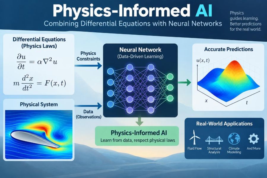
Physics-informed AI sits between these two situations. It uses neural networks for their flexibility while embedding differential equations, conservation laws, boundary conditions, or other scientific knowledge into the learning process.
The goal is not to replace mathematics with artificial intelligence. It is to make mathematical models and learned models work together—especially where data are limited, simulations are costly, and physically credible answers matter.
🧩 The gap between equations and observations
Engineering has long relied on first-principles models: equations derived from physical principles such as conservation of mass, momentum, energy, and charge. These models can be highly interpretable, but they require parameters, initial conditions, and computational effort.
Machine learning begins from the other direction. It learns a mapping from examples, such as temperature readings to predicted heat loss. This can be fast after training, but the model may struggle outside the conditions represented in its training data.
Physics-informed methods narrow this gap by telling a learning algorithm that some behaviors are not optional. Heat should diffuse according to a heat equation; an incompressible fluid should satisfy mass conservation; a structure should respond consistently with its loading and material model.
📜 What a differential equation represents
A differential equation relates a quantity to its rate of change. For instance, if temperature changes through a metal rod, its time rate of change depends on the spatial curvature of temperature and the material’s thermal diffusivity.
One common form of the heat equation is:
∂T/∂t = α ∂²T/∂x²
Here, T is temperature, t is time, x is position, and α describes how readily heat spreads through the material. The notation may look compact, but it encodes a practical statement: sharp temperature differences tend to smooth out over time.
Many engineering systems are governed by ordinary differential equations (ODEs), involving change with one independent variable, or partial differential equations (PDEs), involving change with variables such as space and time.
🧠 What neural networks contribute
A neural network is a flexible function approximator. Given inputs such as position and time, it can produce an estimate of a field quantity—for example, T̂(x,t), an estimated temperature at any queried point.
This is useful because the network produces a smooth, differentiable mathematical function. Modern training software can calculate derivatives of that function with respect to its inputs through automatic differentiation.
That capability creates the key connection. If a network predicts temperature, engineers can differentiate its prediction and check whether it satisfies the heat equation. The equation becomes part of the learning objective rather than a rule checked only after training.
⚙️ The core idea of physics-informed learning
In a standard supervised learning task, a model is penalized when its prediction differs from measured data. A physics-informed neural network, often called a PINN, adds penalties when predictions violate known physical relationships.
A simplified training objective can be written as:
Loss = data loss + physics loss + boundary loss + initial-condition loss
The terms can have different weights. Data loss encourages agreement with measurements. Physics loss evaluates the residual—the amount by which the predicted field fails to satisfy the governing equation. Boundary and initial-condition losses enforce known behavior at edges and starting times.
The trained network seeks a compromise that explains the observations and remains consistent with the imposed physics.
🧪 A simple heat-transfer example
Imagine a thin rod heated at one end. Temperature sensors are available at only a few locations, and some readings are noisy. A conventional neural network could fit those sensor points while predicting unrealistic temperature oscillations between them.
A physics-informed model receives the sparse measurements, the heat equation, and conditions such as a fixed temperature at one end or insulation at the other. It is then discouraged from inventing patterns that would require unphysical heat creation or disappearance.
This does not mean the answer is automatically correct. Wrong thermal properties, unmodeled heat losses, or unreliable sensors can still mislead the model. But the governing equation supplies a strong and useful constraint where observations are absent.
🧭 Initial and boundary conditions are not details
Differential equations rarely define a unique engineering solution on their own. They need information about the system at a starting time and along relevant boundaries.
For a beam, boundary conditions might specify that one end is clamped and the other is free. For fluid flow, they may specify inlet velocity, wall behavior, pressure at an outlet, or periodic conditions. For a battery model, an initial state of charge may be essential.
Physics-informed AI must represent these constraints carefully. A model that satisfies a PDE but applies the wrong boundary behavior can be mathematically polished and physically useless.
🧱 Hard constraints and soft constraints
Constraints can enter training in two broad ways. A soft constraint adds a penalty to the loss when the model violates a condition. The optimizer tries to reduce that penalty, but a small violation may remain.
A hard constraint builds the condition into the model form. For example, if a quantity must be zero at x = 0, the output can be constructed so it always contains a factor of x. The boundary condition is then satisfied exactly.
| Approach | Main strength | Typical challenge |
|---|---|---|
| Soft constraint | Flexible for complex or uncertain conditions | Requires careful loss weighting |
| Hard constraint | Enforces known conditions exactly | Can be difficult to formulate for complex geometries |
The best choice depends on the problem, the certainty of the physical knowledge, and the geometry being modeled.
📏 Why residuals matter
A residual measures the mismatch between a predicted solution and an equation. If a model predicts T̂ for the heat equation, its residual may be:
r(x,t) = ∂T̂/∂t - α ∂²T̂/∂x²
When r is zero everywhere and all conditions are met, the prediction solves the stated equation. In practice, training evaluates residuals at selected points within the domain, often called collocation points.
Residuals provide more than a training signal. Mapping them after training can reveal regions where the model is least faithful to the physics, such as near a sharp boundary layer or a moving front.
📍 Choosing points where physics is checked
Collocation points are locations in space, time, or parameter space where the physics residual is evaluated. Random sampling is common, but it is not always efficient.
A fluid problem may need more points near walls, shocks, interfaces, or regions with steep gradients. A heat problem may need extra attention shortly after a sudden thermal load, when changes are rapid.
Adaptive sampling adds points where residuals are high or where the solution is difficult. This is conceptually similar to mesh refinement in numerical simulation: devote computation where the problem needs it most.
🌊 Fluid mechanics and conservation laws
Fluid models are a natural application because conservation laws are central to trustworthy predictions. For incompressible flow, a velocity field should satisfy a continuity equation expressing that fluid is not spontaneously accumulating or vanishing.
The Navier–Stokes equations add momentum balance, linking velocity, pressure, viscosity, and applied forces. A physics-informed model may learn from velocity measurements while being penalized for violating continuity and momentum equations.
These problems are also difficult. Turbulence, sharp gradients, complex boundaries, and a wide range of spatial scales can make PINN training challenging. Traditional computational fluid dynamics remains indispensable for many high-fidelity applications.
🏗️ Structural mechanics and digital inspection
In structural engineering, measurements may come from strain gauges, accelerometers, cameras, or displacement sensors. The governing relations connect loads, deformation, stress, material stiffness, and geometry.
A physics-informed approach can help infer a displacement or stress field between sparse measurements. It may also support inverse problems, such as estimating an unknown stiffness reduction that could indicate damage.
Such inferences require caution. A localized anomaly can be caused by sensor placement, temperature effects, imperfect supports, or model mismatch—not necessarily a crack. Physics-informed output is evidence to investigate, not an automatic structural diagnosis.
🔋 Batteries, electrochemistry, and hidden states
A battery management system cannot directly measure every internal process. Voltage, current, and surface temperature are observable, but internal concentration gradients and some degradation mechanisms are not.
Electrochemical models use coupled differential equations to describe transport, reaction, and charge balance. Physics-informed learning can combine these relationships with operational data to estimate hidden states or calibrate uncertain parameters.
The attraction is practical: better state estimates can support safer control and maintenance decisions. The limitation is equally practical: real cells vary, age, heat unevenly, and may display mechanisms absent from a simplified model.
🌬️ Surrogate models for expensive simulation
High-fidelity simulation may take minutes, hours, or longer for one operating point. Design optimization, uncertainty analysis, and real-time control can require many evaluations, making direct simulation too slow.
A surrogate model approximates the input-output behavior of the simulator at much lower evaluation cost. Physics-informed training can make a surrogate more plausible between sampled designs and more resistant to obvious violations of known laws.
For example, a surrogate for a heat exchanger may map flow rates and inlet temperatures to outlet conditions and pressure drop. It should still be tested against withheld simulations and, where possible, physical measurements.
🔎 Forward problems and inverse problems
A forward problem starts with a known model and parameters, then predicts the system response. Given conductivity, geometry, and boundary temperatures, compute the temperature field.
An inverse problem runs in the opposite direction: use observed responses to estimate unknown causes. Given measured temperatures, infer conductivity, a heat source, or a boundary heat-transfer coefficient.
Physics-informed AI is especially appealing for inverse problems because sparse data alone may permit many explanations. Physical constraints reduce the set of explanations, although they cannot eliminate uncertainty created by poor observability or an inadequate model.
🎛️ Parameter identification is not parameter truth
When a PINN estimates parameters, its result is conditional on the chosen equations, data, constraints, and training procedure. A fitted parameter may compensate for missing physics rather than represent a true material property.
Suppose a model ignores heat loss through mounting hardware. During calibration, it may produce an inflated thermal conductivity to explain faster-than-expected cooling. The numerical fit can look good while the interpretation is wrong.
Engineers should compare inferred values with feasible ranges, test them under new conditions, and report assumptions. Calibration is valuable, but it is not a substitute for identifiability analysis and engineering judgment.
🧮 Automatic differentiation versus numerical differentiation
Numerical differentiation estimates derivatives from nearby sampled values. It can become noisy, especially when sensor data are sparse or measurement noise is amplified by subtraction.
Automatic differentiation applies the chain rule to the operations used by the neural network. It produces derivatives of the network function accurately to machine precision, subject to ordinary floating-point limitations.
This does not make noisy measurements disappear. Rather, it lets the model calculate derivatives of its smooth learned representation while the physics loss guides that representation toward lawful behavior.
⚖️ The difficult art of balancing losses
Data loss and physics loss can differ dramatically in scale. If the data term dominates, the network may overfit measurements and neglect the equations. If the physics term dominates, it may satisfy an idealized model while missing important observed behavior.
Loss weights may be selected through nondimensionalization, adaptive weighting, gradient-based balancing, or informed experimentation. There is no single setting that works across all equations and datasets.
A useful engineering habit is to monitor each loss component separately. A low total loss can hide one badly satisfied condition if another term is numerically much larger.
📐 Nondimensionalization improves more than notation
Physical variables often have very different magnitudes: pressure may be large, concentration small, and time measured on yet another scale. Such disparities can make optimization poorly conditioned.
Nondimensionalization rescales variables using meaningful reference quantities. Instead of raw values, the model works with ratios such as position divided by characteristic length or temperature change divided by a reference difference.
This process also exposes governing dimensionless groups, such as Reynolds or Peclet numbers. Those groups reveal which mechanisms dominate and can help engineers recognize when a model trained in one regime should not be trusted in another.
🗺️ Geometry is a real modeling challenge
Textbook domains are often rectangles, cylinders, or simple beams. Industrial components have holes, joints, curved surfaces, moving parts, and interfaces between materials.
Representing complex geometry requires careful point sampling and reliable identification of boundaries. Some approaches combine neural networks with meshes, signed-distance functions, coordinate transformations, or domain decomposition.
Geometry errors can undermine an otherwise sophisticated model. If the flow passage, support condition, or material interface is represented incorrectly, the learned solution may faithfully solve the wrong physical problem.
🧱 Domain decomposition for large systems
One network may struggle to represent a solution with different behavior across a large domain. A thermal system could contain smooth regions, thin boundary layers, and abrupt material interfaces all at once.
Domain decomposition splits the problem into subdomains, potentially assigning separate networks to each. Interface conditions then enforce continuity of quantities such as temperature and heat flux, or displacement and traction.
This resembles established numerical methods that divide a complex system into manageable pieces. It can improve representation, but it introduces additional design choices and interface errors to manage.
📊 Data quality still sets the ceiling
Physics constraints do not rescue data that are systematically biased, badly timestamped, or associated with the wrong operating conditions. A temperature sensor with offset error can pull an inferred field away from reality.
Before training, engineers should examine units, synchronization, calibration history, missing data, sensor locations, and plausible operating ranges. This unglamorous work often determines whether a hybrid model becomes useful.
- Separate training, validation, and test conditions where possible.
- Keep records of sensor uncertainty and preprocessing choices.
- Use withheld measurements in physically meaningful regions, not only random points.
- Check whether data cover the regimes where predictions will be used.
🚧 Extrapolation remains a serious risk
Physical constraints can improve behavior beyond the training set, but they do not grant unlimited extrapolation. A model trained on laminar flow should not be assumed reliable in a turbulent regime merely because a continuity equation is enforced.
Similarly, an equation may omit phase changes, damage, contact, chemical side reactions, or control-system effects. In those cases, following the incomplete equation perfectly may still lead to poor predictions.
The practical question is not “Does the model contain physics?” It is “Which physics does it contain, under which conditions is that physics valid, and what important behavior might be missing?”
🧯 Uncertainty needs explicit treatment
Engineering decisions often require ranges, not only point predictions. Inputs, measurements, material properties, and model structure all contain uncertainty.
Possible approaches include repeated training with varied initializations, ensembles, Bayesian methods, interval-based analyses, and propagation of uncertain parameters through the model. Each captures different aspects of uncertainty and carries computational cost.
A small residual is not an uncertainty estimate. It only shows agreement with the specified equation and constraints at evaluated points. Confidence should reflect data coverage, validation performance, model assumptions, and sensitivity to changes.
✅ Validation must test physics and purpose
Validation should go beyond reporting training loss. Compare predictions with independent measurements or trusted simulations at conditions not used for fitting.
Also test quantities that matter to the intended decision. A model may predict average temperature well but miss the peak temperature that governs component life. A flow surrogate may reproduce pressure drop but fail to locate a recirculation zone relevant to mixing.
Useful checks include conservation error, boundary-condition error, residual maps, dimensional consistency, sensitivity trends, and performance near operating limits.
🛠️ When classical numerical methods are better
Finite element, finite volume, and finite difference methods remain powerful tools. When the governing model is well established, geometry is known, and a high-quality mesh is feasible, conventional solvers often provide robust and well-understood results.
Physics-informed neural networks are not inherently faster or more accurate. Training can be difficult for stiff equations, high-frequency solutions, multiscale physics, and large three-dimensional domains.
The hybrid approach is most compelling when it fills a genuine gap: sparse observations, unknown parameters, repeated fast evaluation, data assimilation, differentiable optimization, or coupling between models and measurements.
🔄 PINNs are one option in a wider toolbox
“Physics-informed AI” includes more than PINNs. Engineers may use neural operators to learn families of PDE solutions, hybrid state-space models for time series, machine-learned constitutive laws, or models that correct the discrepancy between simulation and experiment.
A neural operator, for example, aims to learn a mapping between functions, such as boundary conditions and solution fields. This differs from training one network to solve one particular problem instance.
The right architecture follows the task. A broad label should not obscure the actual question: what is known, what is measured, what must be predicted, and what constraints are defensible?
👷 A practical workflow for engineering teams
Start with the decision the model must support. Is the aim fault detection, design optimization, state estimation, or reduced-order simulation? Define the required outputs, acceptable error, operating envelope, and consequences of failure.
- Write down the governing equations, assumptions, and valid regimes.
- Audit data quality, sensor placement, units, and uncertainty.
- Build a simple baseline: a classical model, a data-only model, or both.
- Add physical constraints incrementally and monitor every loss term.
- Validate on withheld conditions and decision-relevant quantities.
- Deploy with monitoring, limits, and a path for retraining or review.
This workflow prevents a common mistake: selecting an advanced method before defining the engineering problem it is supposed to solve.
🚩 Common implementation mistakes
One mistake is treating the governing equation as unquestionable while ignoring its assumptions. Another is applying boundary conditions loosely because they are inconvenient to encode.
Teams also sometimes evaluate only average error, use unscaled variables, or compare against data drawn from the same operating trajectory used in training. These choices can create an optimistic picture of model quality.
Finally, avoid presenting a visually smooth field as evidence of physical correctness. Smoothness is a property of the representation; credibility requires independent checks.
📚 Skills that make the approach accessible
You do not need to become an expert in every branch of AI to begin. The most useful foundation is strong engineering mathematics: differential equations, linear algebra, numerical methods, optimization, probability, and dimensional analysis.
Then learn enough machine learning to understand function approximation, training and validation splits, regularization, gradient-based optimization, and overfitting. Programming frameworks can automate derivatives, but they cannot supply missing physical reasoning.
For working engineers, a small, well-defined problem is often the best starting point: a one-dimensional heat equation, a mass-spring-damper system, or parameter estimation from a controlled experiment.
🔮 Where physics-informed AI is likely to help most
The strongest opportunities tend to involve systems where both data and theory are incomplete on their own. Examples include sensor-limited assets, multi-physics systems, simulation-assisted design, and real-time estimation of quantities that cannot be directly measured.
Its role may be less about producing a single dramatic prediction and more about making routine engineering workflows faster, more interpretable, or better informed. A useful model can prioritize inspections, screen design candidates, estimate states, and identify where further measurement is worthwhile.
Progress will depend on better algorithms, but also on better problem formulation, transparent validation, and teams that understand both the physical system and the limits of the learned model.
🎯 The central principle: learn within the laws that matter
Physics-informed AI works because engineering knowledge can reduce the enormous set of functions a neural network could otherwise learn. Differential equations, conservation laws, and conditions steer learning toward solutions that are compatible with what is already known.
That guidance is valuable, not magical. It must be based on valid assumptions, sound data, appropriate scaling, and testing under conditions that resemble real use.
The most productive mindset is not equations versus AI. It is a deliberate division of labor: physics supplies structure, data supplies evidence, and engineering judgment determines whether the resulting model is fit for purpose.
When neural networks are trained to respect relevant physical laws, they can become more useful engineering models—not because they escape mathematics, but because they are grounded in it. 📐🧠⚙️