
A drawer slide should glide smoothly whether it comes from the first box on a pallet or the ten-thousandth. A car door should close with the same satisfying alignment on every vehicle. A phone charger should fit its port without being loose or requiring force.
None of those outcomes requires every manufactured part to be perfectly identical. In fact, making identical parts would be either impossible or ruinously expensive. Cutting tools wear, materials respond to temperature, and measurement itself has limits.
Manufacturing solves this problem by defining an acceptable range of variation, then using data to understand whether the process stays reliably within that range. That combination of dimensional tolerance and statistical thinking is what makes interchangeable mass production practical.
The mathematics is not merely a quality-department exercise. It guides design decisions, machine settings, inspection plans, supplier agreements, and the cost of every part that reaches an assembly line.
🔧 The manufacturing problem behind “identical” parts
A nominal dimension is the target printed on a drawing, such as a shaft diameter of 10.00 mm. Real shafts do not all measure exactly 10.00 mm. One may be 9.998 mm and another 10.004 mm, even when both are made by a well-controlled process.
Variation comes from many ordinary sources: material batches, machine vibration, tool condition, fixture location, coolant temperature, and operator setup. The engineering question is not whether variation exists; it is whether the variation prevents the part from doing its job.
📏 What a dimensional tolerance actually says
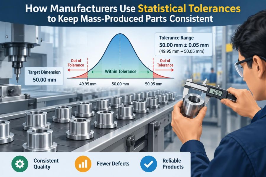
A tolerance states the permissible departure from a nominal value. For example, 10.00 ± 0.05 mm sets a lower specification limit of 9.95 mm and an upper specification limit of 10.05 mm.
Any measured part inside those limits meets that particular dimensional requirement. A tolerance can also be one-sided, such as 10.00 mm minimum, or expressed as limit dimensions such as 9.95–10.05 mm.
🎯 Specifications are not process targets
A frequent misunderstanding is to treat the two specification limits as the desired operating range. They are not. They define the boundary of acceptability, not the place where a healthy process should wander.
If a process is centered at 10.04 mm with an upper limit of 10.05 mm, even modest normal variation will create rejects. A manufacturer generally aims to keep the process mean near a deliberate target, often near the center of the tolerance unless functional needs require an offset.
🧩 Fit and function determine the allowed variation
Tolerances originate in function. A hole and a pin may need clearance so they assemble easily, or interference so the pin stays fixed. A sealing face may need flatness to prevent leakage. A gear feature may need controlled position to mesh quietly.
Designers therefore begin with what the product must do, then translate that need into measurable geometric requirements. A dimension that does not affect function should not automatically receive a very tight tolerance, because unnecessary precision adds cost without improving the product.
🔩 Interchangeability is the mass-production payoff
Interchangeability means a conforming part can be assembled with another conforming part without hand selection or custom fitting. It is why replacement bearings, fasteners, and many appliance components can be produced in separate places and still work together.
In a simple shaft-and-hole assembly, the shaft’s maximum size and the hole’s minimum size determine whether assembly is possible in the worst case. Tolerance decisions thus protect the assembly, not just the individual component.
📐 Bilateral and unilateral tolerances
A bilateral tolerance permits variation on both sides of nominal, as in 20.00 ± 0.10 mm. It is useful when being slightly high or low has similar consequences.
A unilateral tolerance permits variation primarily in one direction, such as 20.00 +0.00/−0.10 mm. This might suit a feature where exceeding the nominal size causes interference, while a slightly smaller value remains functional. The notation communicates design intent directly to production and inspection.
🧭 Geometric tolerances control more than size
Two parts can have the correct measured diameter and still fail to assemble if their axes are tilted, their surfaces are warped, or their holes are in the wrong location. Geometric dimensioning and tolerancing, often called GD&T, controls these features.
Common geometric requirements include position, flatness, perpendicularity, cylindricity, and profile. They define a permissible geometric zone rather than only a plus-or-minus value on a ruler. This gives designers a more direct language for functional relationships.
🌡️ Why every production process varies
Some variation is short-term and random: tiny differences in cutting forces, material grains, or electronic sensor noise. Other variation is systematic, such as a tool slowly wearing, a machine warming after startup, or a fixture being set incorrectly.
Statistical tolerance methods help distinguish these patterns. Random variation may be reduced through process improvement, while a shift or trend often signals a specific assignable cause that should be investigated before it produces nonconforming parts.
📊 The normal distribution as a useful model
For many stable processes, repeated measurements cluster around an average, with fewer observations farther from it. The familiar bell-shaped normal distribution is often a useful approximation for this behavior.
It is a model, not a promise. Some dimensions are skewed, bounded by a physical limit, mixed across different machines, or affected by tool changes. Engineers should inspect the actual data rather than assume every histogram is bell-shaped.
📉 Mean and standard deviation describe a process
The mean is the average measured value and indicates where the process is centered. The standard deviation, usually written as σ for a population or s for a sample, describes the typical spread of values around that center.
A process with a mean of 10.00 mm and a small standard deviation produces a tight cluster. The same mean with a larger standard deviation produces more extreme values and therefore greater risk of crossing specification limits.
🔔 Understanding the “six sigma” spread
For a genuinely normal distribution, the interval from the mean minus three standard deviations to the mean plus three standard deviations contains nearly all observations. Its total width is often called the natural process spread, approximately 6σ.
Manufacturing capability calculations compare this expected spread with the tolerance width. The phrase should not be confused with a blanket claim that every process operating under a “Six Sigma” program has a particular defect rate; definitions and assumptions matter.
⚖️ Tolerance width versus process variation
Suppose a diameter is specified as 10.00 ± 0.06 mm, giving a total tolerance of 0.12 mm. If the process has a 6σ spread of 0.06 mm and is centered, its usual spread occupies about half the available tolerance.
That leaves room for ordinary variation, but it does not eliminate risk. If the process mean shifts, the margin on one side disappears. A capable process needs both a suitably small spread and sensible centering.
🧮 Cp measures potential capability
The capability index Cp compares the specification width with the estimated natural process spread:
Cp = (USL − LSL) / (6σ)Here, USL and LSL are the upper and lower specification limits. A Cp of 1 means the estimated 6σ spread exactly equals the specification width if the process is centered. Higher values indicate more potential room; lower values indicate that the spread is too wide.
Cp does not tell whether the process is actually centered. It can look favorable even while parts are accumulating near one specification limit.
🎯 Cpk reveals centering as well as spread
Cpk considers the distance from the process mean to each specification limit:
Cpk = min[(USL − μ)/(3σ), (μ − LSL)/(3σ)]The smaller side controls the result. A process that is off-center has a Cpk lower than its Cp, sometimes much lower. This makes Cpk especially useful for identifying a process that is technically tight but aimed at the wrong place.
🧪 A hypothetical shaft example
Imagine a shaft specified from 9.95 mm to 10.05 mm. A machine produces a stable average of 10.02 mm, with an estimated standard deviation of 0.01 mm. Its variation is not huge, but the average is closer to the upper limit.
For this example, Cp is 0.10/(6 × 0.01), or about 1.67. The upper-side capability is (10.05 − 10.02)/(3 × 0.01), or 1.00, so Cpk is 1.00. The useful conclusion is not merely a number: recentering the machine could improve practical performance without changing its inherent spread.
📈 Control charts separate noise from signals
A capability index summarizes a period of data. A control chart shows measurements over time, helping engineers see whether the process is stable enough for that summary to be meaningful.
Control limits are calculated from process behavior; they are not the same as specification limits. A point outside a control limit, a sustained drift, or a nonrandom pattern can indicate a process change even when every current part remains within the product tolerance.
🕰️ Why stability comes before capability
Calculating Cpk from a process that is repeatedly adjusted, drifting with temperature, or mixing output from different machines can create a misleading average. The underlying process is not predictable enough for a single standard deviation to represent it well.
Manufacturers commonly establish statistical control first: define rational sampling subgroups, monitor charts, investigate special causes, and then estimate capability from stable data. This order prevents attractive-looking indices from hiding instability.
🔍 Measurement systems can distort the data
A measurement system has its own repeatability and reproducibility. Repeatability concerns whether the same instrument gives similar readings when used repeatedly; reproducibility concerns whether different operators or setups obtain consistent results.
If gauge variation is large relative to the part tolerance, measured process variation contains too much inspection noise. A manufacturer may then reject good parts, accept uncertain parts, or make poor adjustments to a process that was actually healthy.
🧰 Gauge R&R checks the inspection method
A Gauge R&R study evaluates how much observed variation comes from the measurement system rather than from the parts. It typically involves multiple parts, repeated measurements, and more than one appraiser where operator influence is relevant.
The exact acceptance criteria depend on the application, risk, and organizational requirements. The central principle is universal: do not manage a manufacturing process using a ruler, gauge, or test method whose uncertainty is too large for the decision being made.
🏭 Machine-to-machine variation needs attention
A factory may use several machining centers, molding tools, or assembly stations to make the same feature. Each machine can have a slightly different average or spread, even though its individual parts appear acceptable.
Pooling all output may create a wide or multi-peaked distribution that conceals the behavior of each source. Recording machine, cavity, tool, shift, and material-lot information makes it possible to find where variation originates.
🧱 Tolerance stack-up explains assembly risk
An assembly dimension often depends on several individual dimensions. Their variations combine, creating a tolerance stack-up. In a worst-case analysis, all contributors are assumed to reach their most unfavorable limits at once.
Worst-case stack-up is conservative and can be appropriate when failure is unacceptable or parts must assemble in every allowed combination. But it may force very tight component tolerances, because it assumes an extreme combination that may be rare.
📐 Root-sum-square uses statistical combination
When contributors vary independently and approximately randomly, engineers may use the root-sum-square method:
T_RSS = √(T₁² + T₂² + ... + Tₙ²)This predicts that independent variations are less likely to all hit their extreme values in the same unfavorable direction. It can allow more economical tolerances than worst-case analysis, but it is not suitable when dimensions are correlated, distributions are poorly understood, or the consequence of a rare failure is unacceptable.
🔗 Independence is an assumption, not a default
Statistical stack-up relies heavily on independence. That assumption can fail when features are cut in the same setup, shrink together as a molded part cools, or respond jointly to a temperature change.
For example, two dimensions may both grow when a fixture is mislocated. Treating them as independent would underestimate assembly variation. Engineers need process knowledge, not only equations, before selecting a stack-up model.
💰 Tighter tolerances raise production cost
A smaller tolerance may require better machines, slower feeds, finer tooling, more controlled environments, additional inspection, or more scrap and rework. The relationship is not perfectly smooth: a small change can push a process into a different manufacturing method entirely.
The economical choice is not always the widest tolerance, either. Excess variation can cause difficult assembly, warranty issues, sorting costs, and poor product performance. Good tolerance design balances manufacturing cost against functional risk.
🧑💻 Designing for manufacturability early
Design for manufacturability asks whether a part can be made reliably with available processes. Early collaboration among design, manufacturing, quality, and suppliers can identify features that are hard to measure, unnecessary precision, or datum schemes that do not match how the part will be held.
Changing a tolerance on a drawing before production is usually easier than discovering during launch that a dimension demands continual manual adjustment. Functional requirements should be protected; arbitrary precision should be challenged.
📦 Acceptance sampling is not process control
Inspecting a sample from a shipment can support an acceptance decision, especially when testing every item is impractical or destructive. It does not, by itself, control the process that made the shipment.
A sample can miss a localized issue, and sorting finished parts does not remove the cause of variation. Statistical process control focuses upstream: detect meaningful changes and improve the production process before nonconforming output accumulates.
🚫 Common mistakes with capability numbers
- Calculating Cp or Cpk from too little data and treating the estimate as permanent.
- Using specification limits as control-chart limits.
- Ignoring gauge error, rounding, or inconsistent measurement technique.
- Combining different products, cavities, tools, or operating conditions without stratifying the data.
- Adjusting a stable process after every small fluctuation, which can increase variation.
- Using a capability target as a substitute for understanding functional risk.
Indices are useful summaries, not certificates of quality. Their value depends on stable conditions, representative data, suitable distributional assumptions, and a measurement system fit for purpose.
🛠️ Responding when a process shifts
When monitoring reveals a shift, the right response is investigation rather than reflexive knob-turning. Check recent tool changes, material lots, maintenance, fixtures, programs, temperature, measurement setup, and whether the apparent signal is real.
A disciplined corrective action identifies the cause, restores control, documents what changed, and verifies the result over subsequent production. If the process has changed permanently, its capability should be reassessed rather than judged by old data.
🤝 Suppliers need a shared tolerance language
Specifications work best when customer and supplier share the same interpretation of datums, measurement methods, environmental conditions, sampling expectations, and revision status. A drawing alone may not resolve every practical ambiguity.
For critical features, agreeing on how a part will be fixtured and measured can prevent disputes where both parties have plausible measurements but use different reference schemes. Clear communication is part of statistical consistency.
🧠 Statistical tolerance is a decision framework
The deeper value of statistical tolerance analysis is that it connects design intent to process evidence. It asks: What variation can the product tolerate? How much variation does the process create? Can we measure it credibly? What happens when dimensions interact?
Those questions support decisions about redesign, process improvement, tooling investment, inspection frequency, and risk acceptance. The mathematics turns variation from a vague nuisance into a quantity that can be observed, discussed, and managed.
✅ The core principle: control variation, protect function
Mass production succeeds not because every part is exactly alike, but because variation is understood and kept within functional boundaries. Tolerances establish those boundaries; process statistics reveal whether manufacturing can meet them repeatedly.
A robust approach combines functional design, appropriate geometric controls, stable processes, trustworthy measurement, and capability analysis used with its assumptions in view. When any one of these pieces is missing, a reassuring number can conceal an expensive assembly problem.
Statistical tolerances let manufacturers produce parts economically while preserving the fit, performance, and interchangeability that users expect. That is the practical mathematics inside a smooth drawer, a sealed pump, and a reliably assembled product. 📏⚙️📊