
A production line produces shafts with an average diameter exactly at the drawing value. That sounds reassuring—until several parts still fail assembly. The average has hidden a practical problem: individual measurements are spread too far from the target.
A similar situation appears in vibration testing. Two machines can show the same average vibration level, while one runs steadily and the other delivers erratic peaks that point to looseness, wear, or an unstable process.
Engineering decisions rarely depend on an average alone. Designers, test engineers, quality teams, and analysts also need to know how consistently a system behaves. Standard deviation is one of the most useful tools for describing that consistency.
It does not diagnose every cause or guarantee that a process is acceptable. But when it is calculated and interpreted correctly, standard deviation turns a scattered list of readings into a practical measure of variation.
📊 What Standard Deviation Measures
Standard deviation measures how far data values typically lie from their mean, or arithmetic average. A small standard deviation means observations cluster tightly around the mean. A large standard deviation means they are more dispersed.
Its greatest advantage is that it is expressed in the same units as the data. If a sensor records pressure in kilopascals, its standard deviation is also in kilopascals. That makes the result easier to connect to tolerances, operating limits, and physical behavior.
🎯 Why the Mean Is Not Enough
Consider two hypothetical sets of five voltage readings, each with a mean of 10.0 V. Set A is 9.9, 10.0, 10.0, 10.1, and 10.0 V. Set B is 9.2, 10.8, 10.0, 9.5, and 10.5 V.
The means match, but the engineering picture does not. Set A suggests a stable supply over that sample. Set B suggests substantially more fluctuation, which may affect sensitive electronics even though its average is correct.
🔍 Variation Is Often the Engineering Signal
Variation can arise from material properties, tool wear, ambient conditions, operator setup, sensor noise, control-system tuning, or normal random effects. A rising standard deviation can therefore be an early sign that a process is losing consistency.
In other cases, variation is expected. Turbulent flow, rough surfaces, and vibration signals naturally fluctuate. The question is not whether variability exists, but whether its magnitude is compatible with the design purpose and whether its pattern has changed.
🧮 Population and Sample Standard Deviation
The formula depends on what the data represents. Use population standard deviation when the dataset contains every value in the population of interest—for example, every cycle in a short, fully recorded test.
Use sample standard deviation when measurements are a subset used to estimate a larger population, such as 20 parts sampled from a day’s production. This is the usual case in engineering practice.
| Situation | Symbol | Denominator | Purpose |
|---|---|---|---|
| Complete population | σ | N | Describe all recorded values |
| Sample from a population | s | n − 1 | Estimate underlying variation |
➗ The Population Formula
For population values x1, x2, and so on, with mean μ and total count N, the population standard deviation is:
σ = √[ Σ(xᵢ − μ)² / N ]Read it in stages: find each distance from the mean, square the distances, add them, divide by the number of values, then take the square root. The expression inside the square root is the population variance.
🧾 The Sample Formula and Bessel’s Correction
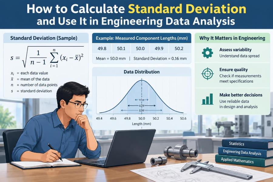
For a sample mean x̄ and sample size n, the sample standard deviation is:
s = √[ Σ(xᵢ − x̄)² / (n − 1) ]Dividing by n − 1 rather than n is called Bessel’s correction. Because the sample mean is estimated from the same data, the deviations are slightly constrained. The n − 1 denominator compensates for the tendency of a sample to underestimate population variability.
For large samples the numerical difference may be small, but the conceptual distinction still matters. Label the calculation clearly so another engineer knows what the reported value represents.
🪜 A Hand Calculation Workflow
A manual calculation is valuable because it reveals what software is doing. Use this reliable sequence:
- List the observations and calculate their mean.
- Subtract the mean from each observation to obtain deviations.
- Square every deviation and sum the squared values.
- Divide by N for a population or n − 1 for a sample.
- Take the square root and report the units.
Keeping a calculation table prevents sign errors and makes a result auditable.
🔩 Worked Example: Shaft Diameter Readings
Suppose a technician measures five shaft diameters in millimetres: 20.01, 19.99, 20.00, 20.02, and 19.98. Treat these readings as a sample from continuing production.
The mean is 20.00 mm. The deviations are +0.01, −0.01, 0.00, +0.02, and −0.02 mm. Their squared values sum to 0.0010 mm².
Dividing by n − 1 = 4 gives a sample variance of 0.00025 mm². The square root gives s = 0.0158 mm, approximately. This describes the observed short-term spread; it does not by itself show whether every part meets a specified tolerance.
📐 Why Squaring the Deviations Matters
If ordinary signed deviations were added, positive and negative values would cancel. Every dataset measured around its own mean would appear to have a total deviation of zero, even when readings were widely scattered.
Squaring solves that cancellation problem and gives larger deviations more influence. This is useful when unusual departures matter, but it also means standard deviation is sensitive to extreme values.
🌡️ Variance Has Different Units
Variance is the average squared deviation before taking the square root. If temperature is measured in degrees Celsius, variance is measured in degrees Celsius squared. If force is measured in newtons, variance is in newtons squared.
Variance is essential in statistical calculations, uncertainty propagation, and modeling. For day-to-day communication, standard deviation is usually more intuitive because it returns to the original engineering unit.
📏 Standard Deviation Is Not a Tolerance
A tolerance is a design requirement, such as a dimension permitted between two limits. Standard deviation is a description or estimate of observed variability. They answer different questions.
A process can have a small standard deviation but be centered away from the nominal target, producing consistently incorrect parts. It can also be centered perfectly at nominal while having a large standard deviation that pushes many parts toward—or beyond—the limits.
🎯 Centering and Spread Must Be Evaluated Together
Imagine a hole specified around a nominal diameter. The process mean indicates where production is centered; the standard deviation indicates how broadly results spread around that center.
Improvement may require shifting the mean, reducing the variation, or both. Adjusting a machine offset can correct centering, while reducing variation may require work on fixturing, cutting conditions, incoming material, temperature control, or measurement method.
📉 Interpreting One, Two, and Three Standard Deviations
For data that is approximately normally distributed, about 68% of observations lie within one standard deviation of the mean, about 95% within two, and about 99.7% within three. This is often called the empirical rule.
These percentages are not universal. Skewed distributions, hard physical limits, mixed operating modes, and outliers can make the rule misleading. Inspect the data distribution before using normal-based interpretations for quality or reliability decisions.
🛎️ The Normal Distribution Is a Model, Not a Default
The familiar bell curve is convenient because its spread is summarized neatly by standard deviation. Many small independent influences can produce approximately bell-shaped results under suitable conditions.
But engineering data may be non-normal. Time-to-failure data are commonly skewed; vibration amplitudes can have intermittent peaks; measurements pooled across multiple machines may form two clusters. Standard deviation remains calculable, yet its “typical spread” interpretation needs context.
📦 How Outliers Can Change the Result
One incorrect value can increase standard deviation sharply. A reading may be an input error, a failed sensor, an unusual but genuine event, or evidence of a changed process. Deleting it merely because it is inconvenient is poor analysis.
Investigate the record: check units, instrument condition, timestamp, setup, and physical plausibility. If there is a documented measurement or transcription error, correct it transparently. If the value is real, retain it and explain its effect.
🧪 Measurement System Variation Comes First
A reported standard deviation combines variation from the item or process with variation from the measurement system. Resolution, calibration, repeatability, operator technique, alignment, and environmental effects can all contribute.
If gauge variation is large relative to the variation you want to detect, the result may mostly describe the gauge rather than the product. A measurement-system study can help separate repeatability and reproducibility issues before process conclusions are drawn.
🕒 Use Time Order Instead of Ignoring It
A single standard deviation compresses a dataset into one number and discards time sequence. That is a limitation when a process drifts, cycles, warms up, or changes after maintenance.
Plot measurements in time order alongside the calculated spread. Ten stable readings followed by ten shifted readings may produce a moderate overall standard deviation, while the time plot reveals a clear change in operating condition.
📈 Standard Deviation in Control Charts
Control charts use estimates of process variation to distinguish routine fluctuation from signals that warrant investigation. Depending on the chart type, control limits may be derived using standard-deviation-based relationships.
Control limits are not the same as specification limits. Control limits describe expected process behavior under a statistical model; specification limits come from functional design requirements. Confusing the two can lead to accepting incapable processes or adjusting stable ones unnecessarily.
🏭 Connecting Spread to Process Capability
Capability indices such as Cp and Cpk compare process spread and centering with specification limits. Under their assumptions, a smaller standard deviation creates more room between the natural process spread and the tolerance boundaries.
These indices are useful summaries, not automatic proof of quality. They require a stable process, an appropriate distributional model or suitable transformation, trustworthy measurements, and a meaningful sampling plan. Capability results should be reviewed with plots and process knowledge.
⚙️ Applications Beyond Dimensional Inspection
Standard deviation appears across engineering disciplines because nearly every measured system varies. Examples include:
- Electrical engineering: voltage ripple, sensor noise, and repeated test outputs.
- Civil engineering: material test results, settlement readings, and load measurements.
- Mechanical engineering: mass balance, torque, surface measurements, and vibration levels.
- Chemical and process engineering: flow, concentration, temperature, and batch consistency.
- Software and systems engineering: response-time variability and repeated benchmark results.
The statistic has the same mathematical meaning in each case, but the acceptable magnitude depends on the physical system and its requirements.
💻 Calculating It in Spreadsheets and Code
Spreadsheets offer built-in standard deviation functions, usually separate functions for a sample and a population. Check the function description rather than relying only on a familiar name, because software labels differ.
In code, use a tested numerical library where possible and explicitly specify the intended degrees of freedom. In many tools, a default standard deviation may use population normalization while another setting applies the sample correction. A one-line calculation still needs engineering judgment about data selection and interpretation.
🧷 Record Units, Basis, and Data Scope
A result such as “standard deviation = 0.12” is incomplete. A useful report states the unit, sample size, time period, source, whether sample or population normalization was used, and any exclusions.
For example: “Sample standard deviation of outlet pressure was 0.12 kPa for 30 one-minute readings collected during steady operation.” This gives reviewers enough context to interpret and reproduce the calculation.
🔄 Compare Like with Like
Comparing standard deviations is meaningful only when the measurements, units, operating conditions, and sampling methods are comparable. A temperature spread during startup should not be casually compared with a spread during steady-state operation.
When variables have very different scales, the coefficient of variation—standard deviation divided by the mean—can sometimes support relative comparisons. It is not suitable when the mean is near zero or when the variable has no meaningful ratio scale, such as temperature in degrees Celsius.
🧩 Subgroups Can Reveal Hidden Causes
An overall standard deviation can be inflated because several distinct conditions have been mixed together: different shifts, material lots, machines, fixtures, operators, or ambient temperatures. The average may hide these groups as well.
Stratify the data before concluding that a process is inherently variable. If each machine is consistent but their means differ, the problem may be machine-to-machine offset rather than within-machine inconsistency. That distinction leads to a different corrective action.
⚠️ Common Calculation Mistakes
Several errors repeatedly produce misleading results:
- Using n when a sample estimate requires n − 1.
- Forgetting the square root and reporting variance as standard deviation.
- Mixing units, such as millimetres and micrometres, in one dataset.
- Rounding every intermediate value too aggressively.
- Calculating spread around a target value when the question requires spread around the sample mean.
- Combining readings from different operating modes without labeling them.
Most of these are prevented by retaining raw data, documenting the method, and checking whether the result has plausible units and scale.
🧠 A Small Standard Deviation Can Still Mislead
A small value looks desirable, but it is not automatically evidence of good performance. It may result from a narrow test range, low instrument resolution, a short observation period, or data that missed important operating conditions.
Likewise, a large standard deviation is not automatically failure. Some systems are intentionally variable, and some signals naturally change with load. Interpretation must be tied to the engineering question, the required performance, and the data-generating conditions.
🗺️ Choose a Sampling Plan Before Calculating
Collecting convenient observations can produce a precise estimate of the wrong condition. Define what period, equipment, loads, shifts, materials, and environmental conditions the result should represent.
Sample enough data to capture meaningful sources of variation, particularly when conditions change over time. There is no universal sample size that fits every engineering problem; risk, cost, process stability, and required decision confidence all matter.
🧭 A Practical Interpretation Checklist
Before acting on a standard deviation, ask a short set of questions:
- What population or operating condition does this dataset represent?
- Is this a sample estimate or a complete population description?
- Are units, measurement quality, and data timestamps reliable?
- Does a histogram or time plot show skewness, clusters, drift, or outliers?
- How does the spread relate to design limits, safety margins, or control needs?
- What physical mechanism could plausibly produce the observed variation?
This connects the calculation to a defensible engineering decision rather than treating it as a standalone score.
✅ The Core Principle for Engineering Decisions
Standard deviation quantifies spread, while the mean describes location. Neither statistic tells the full story alone. Together with plots, measurement-system knowledge, specifications, and process context, they provide a compact but powerful starting point for understanding data.
The strongest use of standard deviation is not simply reporting a number. It is using that number to ask better questions: Is the system stable? Is the variation real? Is it acceptable for the intended function? And what source of variation can be controlled?
Calculate standard deviation carefully, state what it represents, and interpret it alongside the physical process—not apart from it. That habit turns routine measurements into evidence engineers can use with confidence. 📐📊⚙️