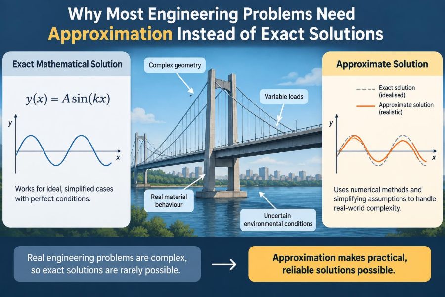

A bridge designer has a deadline, incomplete information about future traffic, and steel whose properties vary slightly from batch to batch. An exact answer to every equation would be impressive—but it would not tell the designer exactly how the finished bridge will behave in every wind gust, temperature change, or loading event.
The same pattern appears in a phone’s battery model, a chemical reactor, a building’s cooling system, and the route followed by a delivery drone. Real systems contain too many interacting details to describe perfectly, and some of the details are not even known when decisions must be made.
That does not mean engineering mathematics is imprecise or careless. It means engineers use mathematics to make controlled, quantified approximations: models that are simple enough to solve and accurate enough for the decision at hand.
Understanding this distinction changes how we judge calculations. The goal is rarely an elegant exact formula. The goal is a dependable prediction, design, or control action within clearly understood limits.
🧭 Exact Mathematics and Engineering Answers Are Different Things
An exact mathematical solution satisfies a set of equations without numerical or algebraic error. For example, the quadratic formula gives an exact expression for the roots of a quadratic equation.
An engineering answer must do more. It must represent a physical system, account for relevant uncertainty, arrive in time, and be accurate enough to support a safe and economical decision. A perfect solution to an unsuitable model is still unsuitable.
This is the central distinction: exactness belongs to the solution of a model; usefulness belongs to the model’s relationship with reality.
🌍 Reality Does Not Arrive as a Closed-Form Equation
A closed-form solution is an expression written using a finite combination of familiar operations and functions. Engineers value such solutions because they reveal relationships clearly and are quick to evaluate.
But physical laws often produce coupled, nonlinear differential equations. Fluid flow around a car, heat moving through a layered wall, and vibration in a flexible machine frame all involve variables that influence one another across space and time.
For many of these systems, no convenient closed-form solution exists. The available choice is not usually “exact formula or failure.” It is a choice among different approximations, experiments, simulations, and safety margins.
🔎 Every Calculation Begins with a Model
A model is a deliberately simplified representation of a system. It selects the features that matter to a question and leaves out features that do not materially change the answer.
Consider estimating the fall time of a dropped tool. A first model may ignore air resistance and treat gravity as constant. For a dense tool falling a short distance, that may be adequate. For a feather or a high-altitude drop, it is not.
Modeling is therefore an act of judgment, not merely equation writing. The engineer asks: what mechanisms dominate, what outputs matter, and what level of error can the application tolerate?
🧩 Simplifying Assumptions Make Problems Solvable
Common assumptions include rigid parts, uniform material properties, steady flow, small deformations, constant temperature, or perfectly mixed fluids. Each assumption removes complexity from the mathematical description.
These assumptions are not claims that reality literally behaves that way. They are hypotheses about whether neglected effects are small enough for the intended result.
- A beam may be treated as one-dimensional when its length is much greater than its cross-sectional dimensions.
- A tank may be assumed well mixed when mixing is rapid compared with the reaction or filling process.
- A structure may be analyzed as linear when deflections are small enough that geometry changes do not significantly alter the forces.
The quality of an approximation depends on whether these assumptions fit the operating conditions.
📏 Scale Determines What Can Be Ignored
Effects that are crucial at one scale can be negligible at another. Surface tension strongly influences a droplet or a microfluidic device, while gravity may dominate the behavior of a large reservoir.
Engineers use dimensionless quantities to compare competing effects. The Reynolds number, for instance, helps compare inertial and viscous effects in a flow. Its value can signal whether a simple laminar-flow assumption is plausible or whether turbulent behavior must be considered.
Scaling analysis often prevents wasted effort. Before building a detailed simulation, it can identify which terms in an equation are likely too small to matter.
➿ Nonlinearity Removes Many Exact Shortcuts
A linear system has a useful property: doubling an input doubles the response, and separate responses can be added together. Many exact techniques rely on this behavior.
Real systems often become nonlinear. Friction can depend on velocity in a nonlinear way, material stiffness can change with strain, chemical reaction rates can vary sharply with temperature, and aerodynamic drag rises rapidly as speed increases.
Nonlinear equations may have multiple possible states, abrupt transitions, or no simple analytical solution. Engineers then approximate them around a chosen operating point or solve them numerically in small steps.
🌊 Turbulence Is a Classic Example of Necessary Approximation
Turbulent flow contains swirling motions across a wide range of sizes. A full physical description would need to resolve many spatial and time scales, especially at high flow speeds or in large systems.
For some small, carefully controlled cases, highly detailed simulations are possible. For practical design of pipes, aircraft components, ventilation systems, or river structures, resolving every swirl is often computationally unrealistic.
Instead, engineers use turbulence models that estimate the average influence of unresolved motion. Those models introduce uncertainty, but they can provide useful pressure losses, forces, and mixing predictions when checked against appropriate data.
🧱 Materials Are Not Perfectly Uniform
Textbook equations may use a single elastic modulus, density, or strength value. Actual materials have manufacturing variation, microscopic defects, aging effects, residual stresses, and sensitivity to temperature or moisture.
A concrete member does not contain identical particles at every point. A composite panel may have local fibre alignment differences. Even a precisely machined metal component has tolerances.
Using one representative property is itself an approximation. Good design accounts for the possible range of properties rather than treating a catalog value as an unchanging fact.
🌦️ Loads and Environments Are Uncertain
Engineering systems are exposed to conditions that cannot be specified exactly in advance: occupancy patterns, wind, rainfall, road roughness, supply voltage, ambient temperature, or operator behavior.
A building cannot be designed for one perfectly known future load history. A thermal system cannot assume its outdoor conditions will remain fixed. The unknowns are part of the problem, not a failure of mathematics.
This is why engineering calculations combine predicted conditions with design cases, allowances, monitoring, and conservative limits where consequences justify them.
🎯 Accuracy Must Be Matched to the Decision
Not all questions need the same precision. During early concept selection, an estimate that distinguishes between a 10 kW and a 1 MW requirement may be more valuable than a slow, highly detailed model.
Later, when choosing component sizes or verifying performance, tighter accuracy may be needed. In a safety-critical application, uncertainty may need formal treatment and independent checking.
The required accuracy is set by consequences, sensitivity, cost, and available margin—not by a general desire for more decimal places.
🧮 Numerical Methods Replace Algebraic Formulas
Numerical methods approximate a continuous problem using a finite set of calculations. A differential equation may be evaluated at discrete time steps, or a physical shape may be divided into many small elements or cells.
The computer does not make the problem exact. It performs a large number of controlled approximations quickly and consistently. The result depends on the equations, input data, numerical scheme, and resolution chosen.
Common methods include finite difference methods, finite element analysis, finite volume methods, and iterative root-finding. Each translates a physical question into a computational procedure.
🕸️ Discretization Turns Continua into Manageable Pieces
Discretization divides a continuous domain into a finite representation. In structural analysis, a component is divided into elements connected at nodes. In computational fluid dynamics, a flow region is divided into cells.
Finer meshes can capture sharper temperature gradients, local stresses, and complex flow features. They also increase memory use, computation time, and opportunities for poor-quality elements or setup errors.
A mesh is not automatically trustworthy because it looks detailed. Engineers test whether refining it changes the important result enough to affect the decision.
⏱️ Time Stepping Introduces Its Own Choices
Transient problems evolve over time: a vibrating motor starts, a battery charges, a control valve moves, or a room temperature changes through a day. Numerical solvers represent this evolution with time increments.
If the step is too large, rapid behavior can be missed or the solution can become unstable. If it is extremely small, the computation may become impractical without meaningfully improving the engineering conclusion.
Appropriate time resolution depends on the fastest important process in the system. A solver should be checked against known behavior, physical expectations, or smaller-step calculations.
⚖️ Approximation Error Has Several Sources
It is useful to separate errors rather than blame “the simulation” as one vague source. Different errors require different remedies.
| Source | What it means | Typical response |
|---|---|---|
| Model-form error | The equations or assumptions omit relevant physics. | Improve the model or narrow its intended use. |
| Input uncertainty | Material properties, loads, or conditions are not known exactly. | Use ranges, testing, and sensitivity analysis. |
| Discretization error | Mesh size or time step is too coarse. | Refine and compare results. |
| Numerical error | Rounding, iteration, or solver behavior affects the result. | Check convergence and solver settings. |
| Human error | Units, geometry, constraints, or interpretation are wrong. | Review independently and use structured checks. |
An exact arithmetic result cannot repair a model-form or input error.
📉 Convergence Is Evidence, Not a Guarantee
Many numerical methods solve a problem iteratively. The solver repeatedly updates an estimated answer until changes become sufficiently small according to selected criteria.
Convergence means the algorithm has settled according to those criteria. It does not prove that the model is physically correct, that the mesh is adequate, or that the boundary conditions represent the real system.
A simulation can converge neatly to the wrong answer. Engineers must therefore examine residuals, result trends, conservation checks, and the plausibility of the physical pattern—not only the solver’s completion message.
✅ Verification Asks Whether the Equations Were Solved Right
Verification concerns the mathematics and implementation. Did the software solve the stated equations correctly? Were the units consistent? Is the mesh sufficiently refined? Does the method reproduce a problem with a known solution?
Useful verification checks include simple hand calculations, limiting cases, symmetry tests, mesh refinement studies, and conservation of mass, energy, or charge where applicable.
For example, a heat-transfer model should behave sensibly if the imposed temperature difference is set to zero. Such tests reveal setup mistakes before a complex result is trusted.
🧪 Validation Asks Whether the Right Equations Were Chosen
Validation compares model predictions with physical measurements or established observations for conditions relevant to the application. It asks whether the model represents reality well enough for its intended purpose.
A validated pump model at one flow range may not be validated at an entirely different fluid temperature or operating regime. Validation is always connected to a stated domain.
Verification and validation are complementary. Verification builds confidence in the calculation; validation builds confidence in the physical representation.
🧭 Boundary Conditions Can Matter More Than Equation Sophistication
Boundary conditions specify how a model interacts with its surroundings: a fixed temperature, applied force, prescribed flow rate, electrical voltage, support constraint, or heat-transfer coefficient.
They are often estimated from incomplete data. A highly advanced structural model with unrealistic supports can be less useful than a simpler model with carefully justified constraints.
Before refining internal details, engineers should ask whether the inputs at the system boundary reflect how the real system is loaded, connected, controlled, and exposed.
📌 Initial Conditions Shape Transient Predictions
For time-dependent systems, the starting state matters. A thermal model needs an initial temperature field; a dynamic model may require initial displacement and velocity; a process model needs initial concentrations.
When a system has a long settling time, an arbitrary initial condition can influence results for much of the simulation. When it settles rapidly, the starting condition may matter only briefly.
Stating initial conditions explicitly makes the limits of a prediction easier to understand and reproduce.
🔬 Sensitivity Analysis Reveals What Deserves Attention
Sensitivity analysis changes an input within a credible range and observes how the output responds. It identifies which assumptions strongly influence the decision and which barely change it.
Suppose a heat-loss estimate changes little when insulation conductivity varies within its expected range but changes greatly with wind speed. Better wind information may be more valuable than further refinement of the material data.
This practice directs measurement effort and engineering review toward the uncertainties that matter most. It also prevents false confidence based on a single set of inputs.
🛡️ Safety Factors Are Not a Substitute for Understanding
Safety factors and design margins help accommodate uncertainty, variation, degradation, and unforeseen deviations. They are essential tools in many engineering contexts.
However, a large arbitrary margin cannot reliably compensate for an incorrect failure mode, an omitted load path, or a model used outside its valid range. It may also create unnecessary cost, weight, or energy use.
A sound approach identifies the uncertainty, estimates its effect where possible, and applies margins consistent with the design method and consequences of failure.
💻 More Computing Power Does Not Eliminate Modeling Judgment
Modern computing makes it feasible to analyze systems that once required crude estimates. That is a major advantage, especially for complex geometry, multiphysics interactions, and repeated design evaluations.
Yet a detailed model requires more assumptions, inputs, and opportunities for misinterpretation. Adding features can obscure the few parameters that actually control the result.
The best model is not necessarily the largest one. It is the simplest model that captures the relevant physics with sufficient confidence for the decision being made.
🏗️ A Beam Calculation Shows the Value of a Simple Model
Imagine estimating deflection in a long, slender steel beam under a modest load. Elementary beam theory may provide a fast prediction using geometry, elastic modulus, support conditions, and loading.
That model may be entirely suitable for preliminary sizing. A more detailed finite element model becomes useful if the beam has complex connections, holes, changing cross-sections, local contact, large deflection, or stresses near a critical feature.
The simple equation is not inferior by default. It is appropriate when its assumptions match the question. The detailed model is justified when it changes a decision or reduces a meaningful uncertainty.
🔋 Battery Predictions Depend on Purpose
A device designer may use a simple equivalent-circuit battery model to estimate voltage sag during normal operation. It can be fast enough for control design and embedded software testing.
A researcher investigating internal temperature gradients, degradation, or extreme charging behavior may need an electrochemical and thermal model with substantially more detail.
Both are approximations. Their value comes from using the right level of representation for the output needed, such as remaining runtime, thermal risk, or long-term capacity change.
🏭 Process Plants Use Balances Before Detailed Simulation
Mass and energy balances are foundational approximations in process engineering. They account for what enters, leaves, accumulates, reacts, or transfers energy within a system.
Before modeling every pipe fitting and mixing zone, an engineer can estimate whether a proposed heat exchanger has enough duty, whether a tank volume is plausible, or whether a process stream can meet a target temperature.
Detailed process simulations add value when phase behavior, control interactions, reaction kinetics, or equipment performance must be resolved. Basic balances remain valuable as transparent checks on those results.
🚗 Control Systems Often Rely on Local Linear Models
A vehicle, robot, or industrial process can be nonlinear over its full operating range. Yet near a chosen operating point, its behavior may be approximated by a linear model.
This local model enables practical controller design and analysis. Engineers then test whether the controller remains acceptable as speed, load, temperature, or position changes.
When one local model is insufficient, designers may use gain scheduling, nonlinear control methods, or multiple operating-region models. The approximation is managed rather than ignored.
⚠️ False Precision Can Mislead a Team
Reporting a result as 12.4837 mm implies a level of certainty that may not exist if the load, material properties, or support conditions are approximate. Extra digits can make an estimate look more authoritative than it is.
Rounding should reflect the uncertainty and decision context. A preliminary estimate might be communicated as an order of magnitude or sensible range, while a manufacturing dimension may require a defined tolerance.
Clear reporting separates computed precision from physical confidence. These are not the same thing.
🧾 Units and Orders of Magnitude Catch Major Failures
Approximation does not mean abandoning rigor. Dimensional analysis checks whether equations combine compatible units and whether the result has the expected physical dimensions.
Order-of-magnitude reasoning is equally powerful. If a small household heater is predicted to warm a large industrial space in seconds, the result deserves immediate scrutiny even if the software ran successfully.
These checks are fast, independent of complex tools, and useful throughout an engineer’s career.
🗣️ Assumptions Should Be Communicated, Not Hidden
A result without its assumptions is difficult to review or reuse. Decision-makers need to know the loading cases, operating range, material data source, neglected effects, and confidence limits behind an important prediction.
Good technical communication does not bury uncertainty in vague caveats. It states what the model can answer, what it cannot answer, and what conditions would require reassessment.
- State the purpose of the calculation.
- List assumptions that materially affect the output.
- Report relevant ranges or margins, not just a single value.
- Identify validation evidence and remaining limitations.
- Recommend the next check when uncertainty remains consequential.
🧠 Common Mistakes When Using Approximate Models
One common mistake is treating a familiar formula as universally valid. A formula may be correct only for a particular geometry, material behavior, flow regime, or range of deformation.
Another is adding complexity automatically. Detailed models can produce attractive visual outputs while concealing weak inputs or untested assumptions.
A third mistake is comparing results only with expectations. Independent checks should be designed to challenge the result: alter the mesh, calculate a simplified case, test a limiting condition, or ask what physical mechanism could make the prediction wrong.
🪜 A Practical Workflow for Responsible Approximation
- Define the engineering decision and required output.
- Identify dominant physics, loads, constraints, and credible uncertainty.
- Start with the simplest defensible model and perform scale checks.
- Select a method with accuracy appropriate to consequences and available time.
- Verify units, implementation, numerical settings, and limiting behavior.
- Validate against measurements or trusted reference cases when possible.
- Perform sensitivity analysis on influential inputs.
- Document assumptions, uncertainty, and the conditions under which the conclusion holds.
This workflow does not guarantee perfect knowledge. It makes uncertainty visible and decisions more defensible.
🌟 The Core Principle: Fit the Model to the Question
Most engineering problems need approximation because real systems are complex, variable, and only partly known. Mathematical exactness alone cannot remove missing data, manufacturing variation, or uncertain future conditions.
Approximation becomes powerful when it is intentional: assumptions are justified, numerical errors are checked, influential uncertainties are explored, and predictions are tested against reality where possible.
The mature engineering question is not “Is this model exact?” It is “Is this model reliable enough, for this decision, under these stated conditions?”
Engineering mathematics succeeds not by pretending reality is perfectly solvable, but by turning unavoidable uncertainty into useful, testable, and responsible approximations. 📐🔧📊