
A machinist measures a shaft as 24.98 mm when its drawing calls for 25.00 mm. A civil engineer receives two survey readings for the same boundary point that differ by a few centimetres. A laboratory sensor reports 101.4 kPa, but its calibration certificate gives a finite accuracy range.
None of these situations means somebody has necessarily made a mistake. Measurements are never perfect copies of reality: instruments have resolution limits, environments change, methods introduce variation, and people must decide how to record and use the result.
Engineering depends on making those limits visible. A number without an indication of its error or uncertainty can look more trustworthy than it really is—and that false confidence can be more harmful than admitting what is not known.
Percentage error and uncertainty provide the mathematical language for this task. They help engineers compare results, judge whether a tolerance is met, select suitable instruments, and communicate decisions honestly.
🎯 What “error” means in engineering mathematics
In measurement science, error is the difference between a measured value and a reference value. If a load cell reads 998 N when a trusted reference load is 1,000 N, its error is −2 N.
The sign matters when diagnosing bias: a negative error indicates an underestimate, while a positive error indicates an overestimate. In many reports, however, engineers use the magnitude of error because the size of the departure is the immediate concern.
Error is not automatically a blunder. A transcription error, wrong unit conversion, or misplaced decimal point is a mistake. Measurement error is the unavoidable difference that remains even when a measurement is carefully performed.
🧭 The reference value problem
To calculate error exactly, a reference or accepted value is required. This may be a calibrated standard, a value supplied by a traceable test facility, a theoretical value in a controlled exercise, or a design value when checking manufactured dimensions.
The true value is an ideal concept: the exact quantity that would be obtained by perfect measurement. In real field work, it is usually unknown. Therefore, engineers often compare against a best available reference rather than claiming to know the true value.
This distinction prevents a common overstatement. A reading can be compared with a calibration standard, but that does not prove the standard represents an error-free truth; the standard itself has uncertainty.
➖ Absolute error: the difference in original units
Absolute error expresses the separation between a measured value and reference value in the same unit as the quantity:
error = measured value − reference valueFor a measured mass of 2.043 kg compared with a reference mass of 2.050 kg:
error = 2.043 − 2.050 = −0.007 kgThe absolute magnitude is 0.007 kg, or 7 g. This form is especially useful when tolerances are specified in physical units, such as ±0.10 mm or ±5 N.
📊 Percentage error: scaling error for comparison
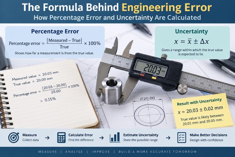
Absolute differences alone can mislead when quantities have different sizes. An error of 2 mm is serious for a 3 mm feature but usually insignificant for a 30 m bridge span. Percentage error scales the difference relative to the reference:
percentage error = |measured − reference| / |reference| × 100%Using the 2.043 kg example:
percentage error = |2.043 − 2.050| / 2.050 × 100% ≈ 0.34%The absolute-value bars mean “take the positive magnitude.” If direction is useful, report signed relative error separately rather than calling a negative result a negative percentage error without explanation.
🔢 Why the denominator must be chosen carefully
In the conventional percentage-error formula, the reference value belongs in the denominator because it defines the scale of the departure. Dividing by the measured value answers a different question and gives a slightly different result.
For instance, comparing 98 V with a 100 V reference gives a 2% percentage error. Dividing by 98 V instead produces about 2.04%, which is a relative difference based on the measurement, not the conventional error relative to the reference.
In specifications, the stated basis matters. A device may be rated as a percentage of reading, percentage of full scale, or percentage of a reference; these are not interchangeable.
🧮 A worked percentage-error example
Suppose a temperature probe is checked in a stable calibration bath whose reference temperature is 80.0 °C. The probe displays 81.2 °C.
absolute error = 81.2 − 80.0 = +1.2 °C
percentage error = |1.2| / 80.0 × 100% = 1.5%
The probe reads high by 1.2 °C, corresponding to a 1.5% error relative to that reference point. This result does not establish its performance at every temperature; sensors can behave differently across their range.
⚠️ When percentage error becomes unhelpful
Percentage error is problematic when the reference value is zero or very close to zero. Division by zero is undefined, and a tiny denominator can make an ordinary absolute difference look like an enormous percentage.
Imagine a pressure difference with a reference of 0.02 kPa and a measurement of 0.04 kPa. The absolute difference is only 0.02 kPa, but the percentage error is 100%. Both facts may be relevant, yet the percentage alone obscures the practical scale.
Near zero, report an absolute error, an uncertainty in physical units, or an error relative to a meaningful full-scale or tolerance value. The chosen basis should match the engineering decision being made.
🔍 Accuracy is not the same as precision
Accuracy describes closeness to a reference value. Precision describes how closely repeated measurements agree with one another. A process can be precise but inaccurate if every reading is consistently shifted from the reference.
Picture darts clustered tightly left of a bullseye: the grouping is precise, but the average position is inaccurate. Widely scattered darts centred around the bullseye may have low precision, even if their average is close to target.
This distinction directs corrective action. A consistent offset may suggest calibration or correction. Scatter may require better environmental control, a more repeatable method, or more careful sampling.
🎲 Random error and repeated readings
Random error causes readings to vary unpredictably around a central value. Electronic noise, small handling differences, vibration, or natural variation in the item being sampled can all contribute.
Repeated measurements help reveal random variation. If five readings of a dimension are 10.01, 10.00, 10.02, 10.01, and 10.00 mm, their spread provides information that one reading cannot.
Averaging repeated independent readings can reduce the effect of random variation on the estimated mean. It does not remove systematic bias, and it should not be used to conceal inconsistent technique or unstable conditions.
📏 Systematic error and measurement bias
Systematic error is a consistent tendency to read too high or too low. A scale with a zero offset, a tape measure stretched by temperature, or a sensor calibrated with an incorrect correction factor can create bias.
Because systematic errors affect readings in a similar direction, taking more measurements does not automatically solve them. One hundred readings from a biased instrument can produce a very stable but still wrong average.
Calibration against suitable standards, control checks, independent methods, and physical understanding of the measurement process are practical ways to detect systematic effects.
🌡️ Environmental conditions change measurements
Temperature, humidity, pressure, electromagnetic interference, vibration, and surface condition can influence measurements. The relevant factors depend on the quantity and equipment: thermal expansion may matter greatly in dimensional metrology, while electrical noise may dominate a low-level voltage test.
An engineering result is therefore not merely a number and unit. It is often a number obtained under stated conditions, using a stated method. Controlling or recording conditions makes the result easier to reproduce and interpret.
Not every possible influence needs a correction. The sensible approach is to identify effects large enough to matter relative to the required tolerance or uncertainty target.
📐 What uncertainty communicates
Measurement uncertainty describes the reasonable doubt associated with a measurement result. It is not a confession that the result is useless; it is a quantified statement of the range within which the value is expected to lie under defined assumptions.
A result written as 12.46 ± 0.03 mm communicates far more than 12.46 mm alone. It tells the reader that the last digits should not be treated as exact and provides a basis for comparing the result with a requirement.
Uncertainty is not necessarily the same as observed error. The actual error may be unknown, while uncertainty estimates the dispersion or range reasonably associated with the stated result.
🧾 Absolute, relative, and percentage uncertainty
Uncertainty can be expressed in several forms. The best form depends on how the result will be used.
| Form | Example | Useful when |
|---|---|---|
| Absolute uncertainty | 5.00 ± 0.02 V | Limits and tolerances use the original unit |
| Relative uncertainty | 0.004 | Calculations and scale-independent comparison |
| Percentage uncertainty | 0.4% | Communicating relative size clearly |
Relative uncertainty is calculated by dividing absolute uncertainty by the measured value. Multiply by 100% to obtain percentage uncertainty:
percentage uncertainty = absolute uncertainty / measured value × 100%🧪 Estimating uncertainty from instrument resolution
For a digital instrument that displays values in steps of 0.01 mm, a simple introductory estimate is often ±0.005 mm, half the smallest displayed increment. This assumes rounding to the nearest increment and does not include other sources.
For an analogue scale, the reading uncertainty depends on graduation spacing, viewing angle, pointer thickness, and judgement. A common classroom estimate is a fraction of the smallest division, but real procedures may specify another method.
Resolution is only one contributor. Calibration limits, drift, repeatability, fixture alignment, and operator technique can make the total uncertainty larger than the display increment.
📜 Manufacturer accuracy specifications need translation
Instrument specifications are compact and easy to misread. A multimeter accuracy statement such as “±(0.5% of reading + 2 digits)” contains two separate contributions: one proportional to the reading and one tied to the least significant display digits.
Suppose the meter reads 12.00 V on a range whose final digit represents 0.01 V. The stated limit would be:
0.5% of 12.00 V = 0.06 V
2 digits = 2 × 0.01 V = 0.02 V
total stated limit = ±0.08 V
This is an illustrative calculation, not a universal meter rule. Always use the specification for the chosen range, operating condition, and calibration status.
➕ Combining uncertainties in sums and differences
When quantities are added or subtracted, their absolute uncertainties are the natural starting point. For a conservative worst-case bound, add their absolute uncertainty magnitudes.
If a length is calculated as 50.0 ± 0.2 mm minus 20.0 ± 0.1 mm, the difference is 30.0 mm. A simple worst-case uncertainty is ±0.3 mm.
This approach is straightforward and cautious. In formal uncertainty work, independent random uncertainty components are often combined using a root-sum-square method rather than simple addition; the method should fit the stated confidence goal and context.
✖️ Combining uncertainties in products and quotients
For multiplication and division, relative or percentage uncertainties are more convenient. A common conservative rule is to add the percentage uncertainties.
Suppose area is found from a rectangle measured as 4.00 ± 0.02 m by 2.00 ± 0.01 m. The area is 8.00 m². The percentage uncertainties are 0.5% and 0.5%, so a simple combined percentage uncertainty is about 1.0%.
The area can therefore be reported approximately as 8.00 m² ± 1.0%, or ±0.08 m². This assumes the dimensions and their uncertainties are treated appropriately; shared influences can create correlation and require more careful analysis.
🧩 Powers amplify relative uncertainty
When a measured quantity is raised to a power, its relative uncertainty is approximately multiplied by the magnitude of that power for small uncertainties. If volume is calculated from a cube side length, V = L³, then the percentage uncertainty in volume is approximately three times that in length.
A 1% uncertainty in side length therefore contributes roughly 3% uncertainty to the calculated volume. This is why small dimensional uncertainty can matter substantially in volume, area, flow, and stiffness-related calculations.
The approximation is most useful when uncertainties are modest. Large uncertainties or strongly nonlinear models deserve direct evaluation using the governing equation or a more formal propagation method.
📈 Root-sum-square and independent contributions
For independent random contributions, engineers often combine standard uncertainty components by root-sum-square (RSS):
uc = √(u₁² + u₂² + ... + uₙ²)The logic is that independent effects are unlikely to all reach their extreme values in the same direction at once. For example, uncertainty due to repeatability, calibration, and resolution may be represented as separate components before combination.
RSS should not be applied mechanically. If two terms arise from the same temperature change or same calibration reference, they may be correlated. Treating them as independent can underestimate the result.
🔗 Correlation: the hidden link between inputs
Inputs are correlated when they tend to move together because of a shared cause. Measuring two lengths with the same tape under the same temperature condition is a simple example: the tape’s scale effect may influence both readings similarly.
In a difference between correlated measurements, a shared effect may partly cancel. In a sum or ratio, it may reinforce or behave differently depending on the equation. This is why uncertainty propagation is not merely a matter of collecting percentages.
For routine work, follow the approved calculation method for the measurement system. For high-consequence or tightly toleranced work, uncertainty analysis should be reviewed by someone competent in the method and its assumptions.
🧠 Type A and Type B uncertainty estimates
A useful classification separates uncertainty estimates by how they are evaluated. Type A evaluation uses statistical analysis of repeated observations, such as estimating spread from repeated measurements.
Type B evaluation uses other information: calibration certificates, manufacturer specifications, prior data, resolution, environmental limits, or physical bounds. Type B does not mean inferior; it means the estimate did not come directly from a repeated-reading statistical calculation.
A complete uncertainty budget commonly includes both. A valve-flow measurement, for example, may combine observed repeatability with a calibration contribution and a temperature-sensitivity contribution.
📋 Building a practical uncertainty budget
An uncertainty budget makes assumptions inspectable. Start with the measurement equation, then list the inputs and plausible uncertainty sources affecting each input.
- Define the quantity being reported and its unit.
- Record the instrument, method, range, and environmental conditions.
- List contributions such as calibration, resolution, repeatability, alignment, and corrections.
- State how each contribution was estimated and whether it is independent.
- Combine contributions using a justified method.
- Report the final result with its uncertainty and coverage statement where applicable.
The budget need not be elaborate for every workshop check. Its depth should be proportional to risk, tolerance tightness, contractual requirements, and the consequence of a wrong decision.
🛠️ Tolerance and uncertainty answer different questions
A tolerance is an allowable range for a part, process, or design requirement. Uncertainty describes doubt in the measurement used to assess that requirement. Confusing the two can lead to poor acceptance decisions.
Consider a component specified as 10.00 ± 0.10 mm. A measurement of 10.08 mm may lie within the drawing tolerance, but if the measurement uncertainty is ±0.05 mm, the actual dimension could plausibly extend beyond the upper limit.
Organisations handle this boundary case through acceptance rules, sometimes called guard bands. The appropriate rule depends on quality requirements, risk allocation, and the governing procedure—not on a universal shortcut.
🚦 Decision risk near specification limits
Whenever a measured result is close to a limit, there are two broad risks. A conforming item may be rejected, or a nonconforming item may be accepted. Measurement uncertainty makes both possibilities more relevant near the boundary.
A guard band moves the acceptance threshold inward from the specification limit. This reduces the chance of accepting a nonconforming item, but it can increase rejection of items that are actually acceptable.
There is no free improvement: reducing one decision risk may raise another. Engineers should make the rule explicit and match it to the application’s consequences.
🧱 A manufacturing example from drawing to decision
Suppose a pin must be between 9.95 mm and 10.05 mm. A micrometer reports 10.04 mm, and the established expanded measurement uncertainty for this use is ±0.02 mm.
The displayed value is inside the drawing limits, but its uncertainty interval overlaps the upper limit. It would be inaccurate to announce that the pin is certainly compliant solely from this measurement.
Possible actions include applying the site’s documented acceptance rule, remeasuring with a lower-uncertainty method, checking instrument condition, or reviewing whether the functional risk actually demands a tighter decision. The correct action depends on the approved quality process.
🧑💻 Significant figures should reflect uncertainty
Reporting too many digits suggests knowledge that the measurement does not support. If a flow is estimated as 18.3746 L/min with an uncertainty of ±0.3 L/min, writing all four decimal places creates false precision.
A clearer report might be 18.4 ± 0.3 L/min. As a practical convention, uncertainty is often rounded to one or two significant figures, and the measured value is rounded to the same decimal place.
Keep extra digits during intermediate calculations to avoid rounding buildup. Round the final reported result only after the uncertainty and reporting convention are established.
🔄 Units and conversions can dominate the error
Many serious engineering failures begin not with difficult mathematics but with an inconsistent unit. A correct percentage calculation cannot rescue a force entered in newtons when a model expects kilonewtons, or a temperature difference mishandled between scales.
Use units at every line of a calculation, especially during conversions. Dimensional analysis—checking that units cancel and the final unit is physically sensible—is a fast way to detect mistakes.
Conversion constants can also have uncertainty in some contexts, although many standard definitions are exact by convention. The key is to understand whether a factor is defined, measured, rounded, or merely assumed.
🚫 Common percentage-error mistakes
Most calculation errors are preventable once the purpose of the calculation is clear. Watch for these recurring problems:
- Using a measured value as the denominator when the task asks for error relative to a reference.
- Dropping the absolute value when reporting an unsigned percentage error.
- Using percentage error without a credible reference value.
- Reporting a huge percentage near zero without also giving the absolute difference.
- Calling a specification limit an uncertainty, or vice versa.
- Rounding early and allowing the rounded value to distort the final percentage.
A formula is only as reliable as the quantities placed into it. Label values before calculating: measured, reference, nominal, tolerance, or uncertainty.
🧰 A reliable workflow for engineering calculations
A disciplined sequence makes routine work faster and easier to audit. First identify what is being measured and what decision the result supports. Then select a reference, method, and instrument capable of meeting the needed uncertainty.
- Write the measurement and unit clearly.
- State the reference value or the reason one is unavailable.
- Calculate signed and/or absolute error as needed.
- Calculate percentage error only when the denominator is meaningful.
- Identify relevant uncertainty sources and combine them appropriately.
- Compare the result with tolerance using the applicable decision rule.
- Report sensible rounding, conditions, and assumptions.
This sequence separates observation from judgement. That separation is valuable when results later need to be reviewed, repeated, or defended.
💻 Spreadsheets and software need engineering checks
Spreadsheets can process large uncertainty budgets and repeated datasets efficiently, but automation does not validate assumptions. A copied formula can reference the wrong cell, use percentages as whole numbers, or hide unit changes behind a clean-looking result.
Build transparent sheets: name inputs, display units, protect key formulas, and test the model with simple hand-calculated cases. A useful check is to change one input slightly and verify that the output moves in the expected direction.
For critical calculations, retain version control, independent review, and enough documentation for another engineer to reconstruct the result.
📝 How to report a result others can use
A strong technical result answers more than “what number did you get?” It identifies the measured quantity, units, method, applicable conditions, and uncertainty expression.
For example: “Pressure at the test connection was measured as 245.2 kPa with an expanded uncertainty of ±1.6 kPa under the stated test conditions.” The phrase “expanded uncertainty” should be accompanied by the relevant coverage basis in formal work.
For informal checks, a simpler statement may be sufficient, but never imply more certainty than the method supports. Clarity allows a colleague to decide whether the result is fit for purpose.
🧭 Choosing the right level of rigor
Not every measurement requires a full statistical uncertainty study. Estimating paint volume for a preliminary job and certifying a safety-critical pressure test do not have the same consequences.
Use a proportionate approach. Higher rigor is justified when tolerances are tight, values are near decision limits, measurements feed design verification, safety or regulatory obligations apply, or the cost of an incorrect decision is high.
Even a simple task benefits from the core habit: know the approximate reliability of the number before relying on it.
✅ The core principle: quantify doubt, then make the decision
Percentage error compares a result with a known or accepted reference. Uncertainty communicates the credible limits of a result when the exact error cannot be known. They work together, but they are not substitutes for one another.
Good engineering measurement means selecting an appropriate reference, using units carefully, recognising random and systematic effects, and matching the calculation method to the decision. It also means resisting the temptation to treat a long decimal display as evidence of accuracy.
The most useful measurement is not always the one with the smallest stated uncertainty. It is the one whose uncertainty is understood well enough for the job at hand.
Engineering error is managed not by pretending measurements are exact, but by expressing their limits clearly and using those limits wisely. 📐🔧📊