
A manufacturing plant is running behind schedule because machines, operators, raw materials, and delivery vehicles must all be coordinated. A bridge designer is trying to reduce material use without compromising safety. An energy manager needs to decide when to charge batteries as electricity demand changes through the day.
None of these problems has one obvious answer. Each contains many possible decisions, competing goals, practical limits, and uncertain conditions. Trying alternatives one by one may work for a small task, but it quickly becomes impossible when the number of choices grows.
This is where optimization algorithms become useful. They provide a disciplined way to search for decisions that are better according to a stated objective, while obeying the constraints that make an engineering design or operation feasible.
Yet optimization is not a magic “best answer” button. Its power depends on the mathematical model, the quality of data, the algorithm selected, and whether the proposed solution still works in the real system.
🧭 What Optimization Really Means
Optimization is the process of choosing the best feasible decision according to a defined measure of performance. That measure might be minimum cost, maximum reliability, lowest energy consumption, shortest completion time, or a carefully weighted combination of several goals.
In engineering mathematics, a problem is often written as minimizing or maximizing an objective function. The adjustable quantities are called decision variables, and the rules they must obey are called constraints.
For example, a logistics planner may choose delivery routes and departure times. The objective may be to minimize travel time, while constraints include vehicle capacity, driver hours, customer time windows, and road accessibility.
🎯 The Objective Function Gives Direction
An algorithm cannot optimize a vague ambition such as “make the system good.” It needs a measurable criterion. The objective function converts an engineering goal into a number that can be compared across candidate solutions.
A structural design objective might combine material mass and estimated fabrication cost. A control problem might penalize deviations from a target temperature as well as excessive actuator movement. The second term matters because constantly switching equipment can create wear even if it controls temperature accurately.
Choosing the objective is a design decision, not merely a mathematical detail. If a model minimizes fuel use but ignores missed deliveries, it may recommend routes that save fuel while failing the operation’s actual purpose.
🧱 Constraints Define What Is Possible
Constraints represent physical laws, safety limits, budgets, geometry, operating procedures, and resource availability. They separate attractive-looking ideas from solutions that can actually be built or operated.
A simple constraint could state that the total weight on a truck cannot exceed its rated capacity. A more involved constraint may express heat transfer through a wall, voltage limits in a power network, or the stress distribution in a mechanical component.
In many real problems, the feasible region—the set of all permitted solutions—is more challenging than the objective itself. A low-cost answer is of little value if it violates a safety margin, misses a deadline, or requires equipment that does not exist.
🔢 Why Complexity Grows So Quickly
Engineering problems become difficult because choices interact. Assigning one job to a machine changes the capacity available for every later job. Altering one beam dimension affects weight, stiffness, cost, vibration behaviour, and connections to other members.
Some problems also contain discrete decisions: select one of several materials, open or close a valve, assign a vehicle to a route, or decide whether to build a facility. The number of combinations can grow extremely rapidly as more choices are added.
Optimization algorithms are powerful because they avoid treating every possible combination equally. They use mathematical structure, estimates, and search rules to focus effort on promising parts of the decision space.
📏 Continuous and Discrete Decisions
A continuous variable can take values over a range, such as pipe diameter, motor speed, or the thickness of insulation. A discrete variable takes separate choices, such as a standard bolt size or a yes-or-no maintenance decision.
Continuous optimization is often easier when the objective and constraints are smooth mathematical functions. Discrete and mixed problems are usually harder because a tiny change is not always possible: a fleet vehicle cannot be assigned “halfway” to two routes.
Many industrial models are mixed: production quantities may be continuous approximations, while machine start-up decisions are binary. Recognizing the variable type early helps engineers choose a suitable method.
📈 Linear Programming and Its Practical Reach
Linear programming applies when the objective and constraints can be represented by linear equations or inequalities. Despite the name, it can describe substantial planning problems involving blending, production, transportation, staffing, and network flows.
Suppose a factory must decide quantities of several products. Material availability, machine hours, and storage limits can often be expressed linearly, while the objective is to maximize contribution margin or minimize operating cost.
Its strength is not only speed. Linear programming methods can often handle large, structured models and provide useful information about which constraints are binding—meaning they actively restrict improvement.
🧩 Integer Programming Handles Yes-or-No Choices
Integer programming requires some variables to be whole numbers. Binary variables, restricted to zero or one, represent decisions such as selecting a site, switching on a generator, or assigning a technician to a shift.
These models are especially useful for scheduling and network design, but they can demand significant computation. An algorithm may need to explore and eliminate many branches of possible choices before proving that a solution is optimal.
For large practical models, a solver may return an excellent solution with a stated gap between its result and a mathematical bound. That can be operationally sufficient, provided the team understands that “best found” is not always the same as “proven globally best.”
🌀 Nonlinear Optimization Reflects Real Physics
Many engineering relationships are nonlinear. Aerodynamic drag changes nonlinearly with speed, chemical reactions depend nonlinearly on concentration and temperature, and structural deflection may become nonlinear at large deformation.
Nonlinear optimization can represent these effects more faithfully than a linear approximation. However, it may have several local optima: points that are better than nearby alternatives but not necessarily the best solution across the entire feasible region.
That distinction matters. A method that starts from different initial designs may converge to different answers, so engineers should test starting points, inspect physical plausibility, and avoid overstating certainty.
🏔️ Local Optima and Global Optima
Imagine hiking through fog while trying to reach the lowest point in a landscape. Walking downhill leads to a nearby valley, but another valley elsewhere may be lower. This is the central difficulty of non-convex optimization.
A local optimum cannot be improved by small nearby changes. A global optimum is the best feasible point in the entire search space. Convex problems have favourable structure: under appropriate conditions, a local optimum is also global.
When a model is non-convex, an engineer may use multiple initial points, global search methods, physical insight, or simplifications. The correct response is not to distrust the result automatically, but to describe its scope honestly.
🧬 Heuristics Search When Exact Methods Struggle
Heuristics are practical rules or search strategies intended to find good solutions quickly without guaranteeing the absolute optimum. They are often valuable for complex routing, layout, scheduling, and design-space exploration problems.
Methods inspired by natural processes, such as genetic algorithms and particle swarm approaches, can explore varied candidate solutions. Simulated annealing occasionally accepts a worse move to avoid becoming trapped too early in a local region.
These approaches are useful tools, not universal replacements for mathematical optimization. Their results can depend on tuning, random seeds, and stopping criteria, so repeat runs and benchmark comparisons are sensible.
⚙️ Gradient Methods Use Slope Information
For differentiable problems, gradients indicate how the objective changes when variables change. Gradient-based methods use this slope information to move efficiently toward improvement.
They are widely used in parameter estimation, optimal control, shape design, and machine learning. Their efficiency is especially valuable when each model evaluation involves an expensive simulation.
But gradients must be reliable. Numerical noise, discontinuities, poor scaling, or an inaccurate derivative can send the algorithm in an unhelpful direction. Checking gradients on smaller test cases is often worth the time.
🧪 Simulation-Based Optimization Connects Models to Behaviour
Some objectives cannot be calculated by a simple formula. An engineer may need a computational fluid dynamics model to estimate pressure loss, a finite element model to estimate stress, or a discrete-event simulation to estimate queueing delays.
Simulation-based optimization repeatedly adjusts inputs, runs the model, and evaluates the outcome. It can tackle highly realistic systems, but computational cost becomes a central concern when one simulation takes minutes or hours.
Common responses include parallel computing, simplified models, surrogate models, and careful selection of which designs to evaluate. More detail is not always better if it makes the optimization too slow to support a real decision.
🪞 Surrogate Models Can Speed Up Expensive Searches
A surrogate model is a faster approximation of a costly simulation. It learns or fits the relationship between design inputs and outputs using a limited set of high-fidelity evaluations.
For instance, during an early aircraft component study, a surrogate may estimate drag and stress trends across many geometry variations. Promising designs are then verified with the more detailed simulation.
The risk is extrapolation: a surrogate may be unreliable outside the range of data used to construct it. Good practice includes tracking prediction uncertainty where possible and repeatedly validating selected candidates with the original model.
⚖️ Multi-Objective Problems Rarely Have One Winner
Engineering often involves competing objectives. Lowering weight may increase cost. Increasing safety margin may reduce usable capacity. Faster delivery may require more vehicles or energy.
Rather than forcing all objectives into one score immediately, multi-objective optimization can identify a Pareto frontier. On this frontier, improving one objective requires worsening at least one other objective.
This output changes the conversation. Instead of asking an algorithm to make a managerial or ethical trade-off invisibly, decision-makers can compare transparent alternatives: lower cost with higher emissions, for example, or higher reliability with greater capital expense.
📊 A Simple Comparison of Algorithm Families
| Approach | Best suited to | Key strength | Main caution |
|---|---|---|---|
| Linear programming | Linear allocation and flow problems | Fast, interpretable solutions | Requires linear representation |
| Integer programming | Scheduling, selection, assignment | Captures discrete choices | Can become computationally difficult |
| Nonlinear programming | Design and physical-process models | Represents nonlinear behaviour | May find only a local optimum |
| Heuristics | Large, irregular search spaces | Flexible and often practical | No general guarantee of optimality |
| Simulation optimization | Complex system behaviour | Uses realistic models | Evaluation cost can dominate |
🏗️ Structural Design Shows Both Power and Limits
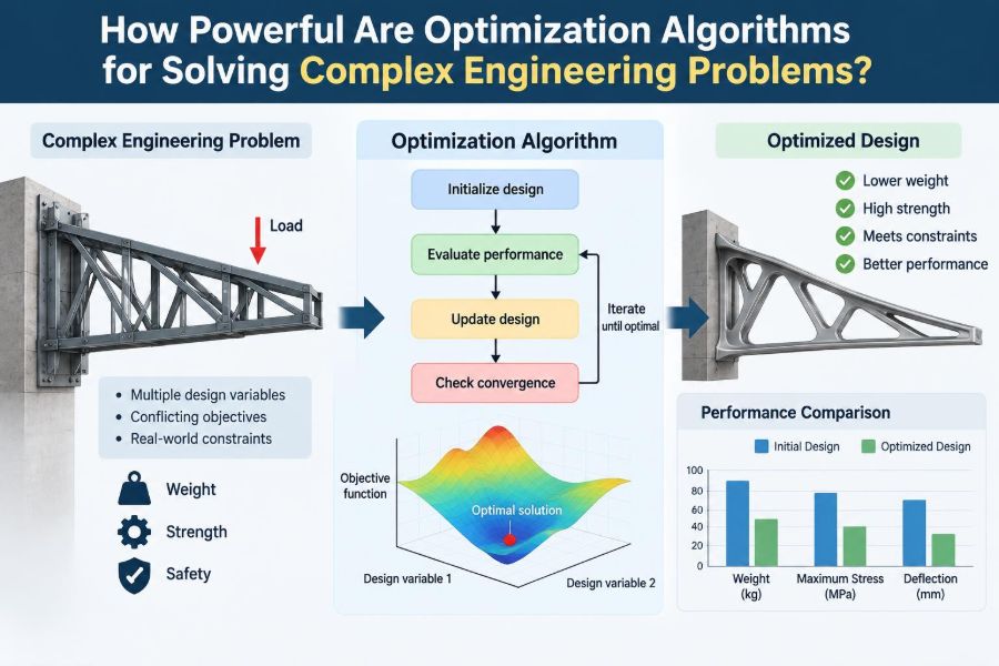
Consider a hypothetical truss design problem. Variables might include member cross-sectional areas, while constraints include stress limits, displacement limits, buckling resistance, available sizes, and connection requirements.
An optimization model can identify designs using less material than an initial hand-designed alternative. This is valuable because material reduction can affect cost, transport, fabrication, and embodied environmental impact.
However, the result still needs engineering review. Fabrication complexity, inspection access, corrosion allowance, fatigue loading, and construction tolerances may not be fully captured in an early mathematical model.
🚚 Routing and Scheduling Turn Operations Into Decisions
Routing problems determine how vehicles, robots, tools, or information should move through a system. Scheduling determines when tasks should occur and which resource should perform them.
In a maintenance operation, optimization may group work orders geographically, account for technician skills, reserve time for urgent calls, and reduce unnecessary travel. The model must still allow for uncertain job duration and real-time disruptions.
The best schedule on paper can fail if it assumes every task begins exactly on time. Robust operational plans usually include slack, priorities, and rules for revising decisions when conditions change.
🔋 Energy Systems Need Decisions Across Time
Energy optimization often links decisions across hours, days, or seasons. Charging a battery now changes what energy is available later. Starting a generator may have minimum operating times. Heating a building early can affect later comfort and demand.
These problems balance supply, demand, storage, cost, emissions, equipment limits, and reliability. Forecasts for renewable generation and load introduce uncertainty, making a single fixed plan less dependable.
Rolling-horizon optimization is a useful approach: optimize using current forecasts, implement only the near-term action, then update the model as new information arrives. This resembles navigation systems that recalculate after traffic changes.
🤖 Control Optimization Makes Systems Respond
Optimal control chooses actions over time to guide a dynamic system. Examples include regulating process temperatures, steering autonomous equipment, and managing battery charging.
Model predictive control repeatedly predicts future behaviour over a finite horizon, chooses a sequence of actions, applies the first action, and then solves again after receiving new measurements. It can manage constraints explicitly, which is a major practical advantage.
Its performance depends on a sufficiently accurate model and timely computation. If sensors are faulty or the process changes beyond the model’s assumptions, conservative safeguards and fallback controls remain necessary.
🌦️ Uncertainty Changes What “Best” Means
Measurements are noisy, demand forecasts can be wrong, and equipment may not perform exactly as expected. Optimizing only for average conditions can produce fragile designs that work well in a spreadsheet but poorly under variation.
Robust optimization seeks solutions that remain acceptable across a defined range of uncertain inputs. Stochastic optimization uses probabilistic descriptions when meaningful probability information is available.
Both approaches involve trade-offs. Greater protection against uncertainty can increase cost or reduce nominal performance. The aim is not maximum caution at all times, but a level of resilience appropriate to the consequences of failure.
🧮 Data Quality Can Overpower Algorithm Quality
A sophisticated algorithm cannot correct an objective built on inaccurate demand, outdated equipment capacities, missing failure modes, or inconsistent units. The phrase “garbage in, garbage out” is blunt, but the underlying warning is sound.
Before trusting results, teams should verify data sources, units, assumptions, time periods, and definitions. A capacity recorded as a theoretical maximum is not the same as dependable operating capacity.
Data gaps do not always prevent optimization. They may require scenario analysis, conservative assumptions, or a simpler model whose uncertainty can be explained clearly.
🔍 Model Validation Is More Than Checking Code
Verification asks whether the model and software implementation solve the equations intended. Validation asks whether those equations represent the real decision problem well enough for their intended use.
Useful checks include comparing predictions with historical operating data, testing known special cases, asking domain experts to review assumptions, and inspecting whether recommended decisions make physical sense.
A result that appears mathematically precise can still be operationally wrong. For example, a schedule might be optimal under assumed travel times yet ignore a site-access restriction known by field staff.
🧷 Sensitivity Analysis Explains the Result
Sensitivity analysis investigates how the recommended solution changes when inputs or assumptions change. It answers questions such as: What happens if demand rises? Which cost estimate matters most? At what capacity does a new machine become worthwhile?
This is particularly valuable when decisions are expensive or difficult to reverse. A design that remains effective across plausible assumptions is usually more persuasive than one that wins only under a narrow set of inputs.
For linear models, shadow prices can offer insight into the value of relaxing a constraint locally. They should be interpreted carefully: they are model-based marginal values, not permanent market prices or universal engineering facts.
🧑💻 Humans Still Define the Problem
Optimization does not replace engineering judgement. People choose what counts as success, identify constraints, interpret results, and decide whether a recommendation is acceptable in a social, operational, and safety context.
Stakeholder input is especially important when objectives conflict. A model cannot independently decide how to value customer inconvenience, worker workload, environmental impact, or rare but severe failure consequences.
The strongest workflow combines domain knowledge with computational search. Engineers use algorithms to reveal options and trade-offs that would be difficult to see manually, then apply professional judgement to select and implement a responsible option.
⚠️ Common Mistakes That Weaken Optimization Projects
- Optimizing the wrong metric: reducing one cost while neglecting reliability, quality, or service requirements.
- Missing constraints: producing an answer that is mathematically feasible but physically or procedurally impossible.
- Using false precision: reporting many decimal places when input uncertainty is large.
- Assuming a solver status proves reality: a solved model may still contain poor assumptions.
- Ignoring implementation: recommending changes without considering training, maintenance, approvals, or operator acceptance.
These failures are often more consequential than choosing between two competent algorithms. Good problem formulation deserves serious engineering effort.
🛠️ A Practical Workflow for Starting Well
- State the decision to be made in plain language.
- Define success measures and identify non-negotiable constraints.
- List decision variables, available data, uncertainty, and required time scale.
- Build the simplest model capable of answering the immediate question.
- Test it on small cases and compare outputs with engineering expectations.
- Choose an algorithm that fits the model structure and computational budget.
- Validate proposed actions, analyse sensitivity, and plan how results will be monitored.
This sequence prevents a common trap: building a technically impressive model before confirming that it answers a useful operational question.
📦 Scaling Up Requires More Than Faster Hardware
Large optimization projects can involve millions of variables, long planning horizons, or repeated simulation runs. Better processors and cloud resources can help, but model reformulation is often equally important.
Engineers may decompose a large problem into connected subproblems, relax selected constraints to obtain bounds, aggregate similar decisions, or solve a detailed model only where it adds value. Problem-specific structure is an asset.
A smaller model that is updated frequently and understood by operators may outperform a massive model that is too slow, opaque, or fragile to use.
🧠 Explainability Builds Trust in Recommendations
Decision-makers need more than a final number. They need to know which constraints drive the plan, what trade-offs were made, what assumptions matter, and when the recommendation should be reconsidered.
Clear visualizations, scenario comparisons, and plain-language summaries make optimization usable beyond the modelling team. Explainability also exposes errors: if nobody can describe why a solution changes, the model may need closer inspection.
For safety-critical or high-consequence applications, transparency should include limits of the model and defined escalation paths when real conditions fall outside the analysed range.
🔐 Safety, Fairness, and Responsible Boundaries
An algorithm follows the goals and constraints it receives. If worker fatigue, accessibility, emissions, or safety buffers are omitted, the model may systematically trade them away for a narrow efficiency measure.
Responsible optimization treats critical requirements as explicit constraints or carefully assessed objectives. It also considers whether historical data may encode uneven service levels or biased operating practices.
Automation should not remove accountability. Engineers and organizations remain responsible for monitoring outcomes, investigating unexpected effects, and overriding automated recommendations when necessary.
🚀 Where Optimization Delivers Its Greatest Value
Optimization is most valuable when decisions are repeated, choices are numerous, trade-offs are real, and performance can be measured. Production planning, network operation, design sizing, inventory allocation, route planning, and process control are common examples.
It is less useful when the objective is fundamentally undefined, relevant data are unavailable, or a simple engineering rule already solves the problem reliably. Not every decision needs an elaborate model.
The key question is not “Can this be optimized?” but “Will optimization improve this decision enough to justify the modelling, computing, validation, and change-management effort?”
🌟 The Core Principle: Powerful Search Needs Sound Engineering
Optimization algorithms can explore complex choices at a scale and speed that unaided human reasoning cannot match. They can reduce waste, expose trade-offs, coordinate constrained resources, and help engineers compare alternatives systematically.
But their output is only as meaningful as the problem formulation. A trustworthy result requires a relevant objective, realistic constraints, suitable algorithms, credible data, testing under uncertainty, and review by people who understand the physical system.
The most powerful use of optimization is therefore not blind automation. It is structured decision-making that combines mathematics, computation, evidence, and engineering judgement.
Optimization algorithms are powerful because they turn complex engineering choices into testable, transparent trade-offs—but sound models and responsible human oversight determine whether those choices work in practice. 📐⚙️🌍