
A bridge deck warms unevenly in the sun. An electric vehicle battery heats while it delivers power. A factory operator adjusts one valve and watches pressure change, even though temperature and flow rate are also moving.
These are not one-variable problems. The outcome depends on several inputs at once, and an engineer often needs a focused question: what happens if I change this one input right now, while holding the others fixed?
That question is the practical heart of a partial derivative. It turns a complicated relationship into a local measure of sensitivity—one that can guide design choices, safety margins, control systems, and optimization.
The notation can look abstract at first. But once it is connected to slopes, measurements, and engineering models, partial differentiation becomes a useful language for describing real systems.
🧭 The central idea: change one input at a time
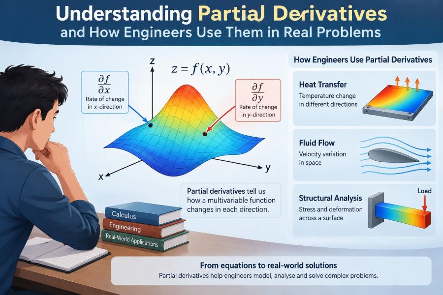
A partial derivative describes how an output changes with respect to one chosen input when the other inputs are treated as constant. If a quantity z depends on x and y, written as z = f(x, y), then ∂z/∂x asks how z changes as x changes while y is fixed.
The curled symbol ∂ is read “partial.” It signals that the function has multiple independent variables, unlike an ordinary derivative such as dy/dx.
📈 From an ordinary slope to a partial slope
For a one-variable function, a derivative is the slope of a curve. For example, if distance depends only on time, the derivative of distance with respect to time is velocity.
With two inputs, the graph is usually a surface rather than a curve. A partial derivative is the slope of that surface along one direction. Holding y constant and changing x traces one curve across the surface; ∂f/∂x is the slope of that curve at the point of interest.
🧮 Reading the notation without mystery
For a function f(x, y), engineers commonly write fx, ∂f/∂x, or ∂xf for the partial derivative with respect to x. Similarly, fy means ∂f/∂y.
Subscripts matter. The expressions ∂f/∂x and ∂f/∂y generally describe different physical effects and may have different units. Always read the denominator as the input being varied.
✏️ A first calculation by holding variables constant
Suppose f(x, y) = 3x²y + 4y³ − 7x. To find ∂f/∂x, treat y as a constant, exactly as you would treat the number 5 in ordinary differentiation:
∂f/∂x = 6xy − 7To find ∂f/∂y, treat x as constant instead:
∂f/∂y = 3x² + 12y²The rule is simple, but the interpretation is richer: each result tells how the output responds in a particular direction through the input space.
🏞️ Visualizing a surface with cross-sections
Imagine a topographic map of a hill, where height is f(x, y). Walking east while keeping your north–south location fixed gives one directional slope. Walking north while keeping east–west position fixed gives another.
Those two slopes are partial derivatives. A steep eastward slope does not imply a steep northward slope. This distinction is why a single “rate of change” is insufficient for systems with several inputs.
📍 Evaluating a derivative at an operating point
A derivative formula becomes most useful when evaluated at a specific state. If fx = 6xy − 7, then at x = 2 and y = 3, fx = 29.
This says that near that operating point, a small one-unit increase in x, with y held at 3, changes f by approximately 29 units. The word near matters: derivatives are local descriptions, not automatic predictions over large changes.
📏 Units give partial derivatives physical meaning
Units are one of the fastest ways to check whether a partial derivative makes sense. If pressure P depends on temperature T and volume V, then ∂P/∂T has units of pressure per temperature, while ∂P/∂V has units of pressure per volume.
| Derivative | Meaning | Typical units |
|---|---|---|
| ∂P/∂T | Pressure sensitivity to temperature at fixed volume | Pa/K |
| ∂P/∂V | Pressure sensitivity to volume at fixed temperature | Pa/m³ |
| ∂T/∂x | Temperature variation along a position coordinate | K/m |
A result with incompatible units usually points to a missing conversion, a mistaken variable, or an incorrect model.
🌡️ Thermodynamics: pressure, temperature, and volume
Thermodynamics is full of partial derivatives because state variables are connected. For an ideal gas, P = nRT/V. At fixed volume, increasing temperature increases pressure, so ∂P/∂T = nR/V.
At fixed temperature, increasing volume decreases pressure, giving ∂P/∂V = −nRT/V². The negative sign is not decorative: it captures an inverse relationship under the stated condition.
🔒 Why “held constant” is a real engineering condition
The phrase “hold other variables constant” is not merely a calculus instruction. It defines the experiment, model, or control condition. In a sealed rigid vessel, volume is approximately fixed; in a piston arrangement, it may not be.
Using ∂P/∂T at constant volume to describe a freely expanding gas would be misleading. Before interpreting a partial derivative, ask which variables are physically constrained and which are free to respond.
🔥 Heat transfer and temperature gradients
Temperature inside a solid may vary with position: T(x, y, z). The derivative ∂T/∂x measures how rapidly temperature changes along the x-direction, while holding y and z fixed.
Heat tends to flow from hotter to cooler regions. In simple conductive models, the heat-flux component in the x-direction is proportional to −∂T/∂x. Engineers use these gradients when assessing insulation, electronics cooling, furnaces, and thermal stresses.
⚡ Electrical fields from voltage changes
Voltage can vary across space, written V(x, y, z). The electric field points toward decreasing voltage, and its components are related to negative partial derivatives: Ex = −∂V/∂x, with equivalent expressions for y and z.
This lets engineers move from a scalar map of voltage to a directional field that predicts forces on charges. It is a foundational connection in electromagnetics, sensors, insulation design, and circuit-field simulations.
🌊 Fluid flow: velocity changes across a channel
In a pipe, fluid velocity is often higher near the center than near the wall. If u(y) describes velocity across a channel, ∂u/∂y measures how quickly velocity changes with transverse position.
That velocity gradient is linked to shear: adjacent layers moving at different speeds exert tangential forces on one another. The details depend on the fluid model and geometry, but partial derivatives provide the language for expressing the local variation.
🏗️ Stress and deformation in structures
Structures deform differently from point to point. A displacement field may be written u(x, y, z), where u represents movement in one coordinate direction. Partial derivatives of displacement describe local stretching, compression, and rotation.
Finite element software calculates related quantities across many small elements. The software automates the arithmetic, but the interpretation remains essential: large gradients can identify regions where deformation changes sharply and where a design may require closer attention.
🚗 Vehicle performance and design trade-offs
A vehicle’s energy use can depend on speed, mass, road grade, ambient temperature, tire pressure, and driving strategy. A partial derivative such as ∂E/∂m estimates how energy use changes with mass near a stated operating condition.
This does not mean mass has one universal penalty. The sensitivity can differ in city traffic, steady cruising, uphill travel, or regenerative braking. Partial derivatives expose these local trade-offs rather than hiding them inside one average number.
🏭 Process control uses local sensitivities
Industrial processes often have outputs such as concentration, temperature, level, or pressure and inputs such as valve position, heater power, and feed rate. Around a normal operating point, partial derivatives approximate how each input affects each output.
These local sensitivities help engineers tune controllers and decide which actuator has the most direct influence. Real plants also have delays, noise, nonlinear behavior, and coupling, so a derivative-based model is usually one part of a broader control analysis.
🧩 The gradient collects all first partial derivatives
For a scalar function f(x, y, z), the gradient is the vector of first partial derivatives:
∇f = (∂f/∂x, ∂f/∂y, ∂f/∂z)The gradient points in the direction of the steepest local increase of f. Its magnitude gives the steepness in that direction. In engineering, gradients describe temperature change, pressure change, concentration change, potential fields, and objective-function sensitivity.
🧭 Directional derivatives answer more realistic questions
Changing only x or only y is useful, but many physical changes occur along a combined direction. A directional derivative measures the rate of change as the inputs move together in a chosen direction.
For a unit direction vector u, the directional derivative is ∇f · u. This dot product combines the relevant partial derivatives and weights them according to the direction of motion or adjustment.
🔄 Second partial derivatives reveal curvature
First partial derivatives describe local slopes. Second partial derivatives describe how those slopes change. For example, ∂²f/∂x² indicates curvature in the x direction.
Curvature matters in optimization, stability analysis, vibration approximations, and nonlinear model behavior. A slope near zero may indicate a flat region, a local peak, a local valley, or a saddle-shaped surface; second derivatives help distinguish these cases.
🪢 Mixed partial derivatives capture interaction
A mixed partial derivative, such as ∂²f/(∂y∂x), asks how the x-sensitivity changes as y changes. It captures interaction between inputs.
For a smooth enough function, the two orders of differentiation are equal: ∂²f/(∂y∂x) = ∂²f/(∂x∂y). In physical terms, this may reveal that the effect of one design variable depends on the level of another.
🎯 Optimization: finding better designs
Engineers often minimize cost, mass, energy loss, or error, while maximizing reliability, strength, output, or efficiency. If f is an unconstrained objective function, candidate stationary points occur where its first partial derivatives are zero.
That condition is only a starting point. Engineers must classify the point, check constraints, evaluate feasibility, and consider uncertainty. A mathematical optimum that violates a temperature limit, manufacturing tolerance, or safety requirement is not an acceptable design.
🧱 Constraints change the problem
Most real designs have limits: a beam must fit a space, a vessel must withstand pressure, and a motor must operate within current and temperature ratings. Variables cannot always be altered independently.
Methods such as Lagrange multipliers formalize optimization with equality constraints. More generally, constrained numerical optimization handles bounds and complex requirements. The key lesson is that partial derivatives describe sensitivity, while constraints determine which changes are actually allowed.
📐 Linear approximation for small changes
Near (x, y), a small output change can be approximated by:
Δf ≈ (∂f/∂x)Δx + (∂f/∂y)ΔyThis is the multivariable version of using a tangent line. It is useful for quick estimates, tolerance analysis, and control, provided the input changes are small enough and the function is sufficiently smooth near the operating point.
🎛️ Sensitivity analysis and tolerances
No manufactured part is exact. Dimensions, material properties, sensor readings, and loads all vary. Partial derivatives estimate which variations affect performance most strongly.
If an output has a large derivative with respect to a particular parameter, a small error in that parameter can matter. Engineers may then tighten its tolerance, improve measurement, redesign for lower sensitivity, or include a wider safety margin.
🧪 Analytical, numerical, and experimental derivatives
An analytical derivative comes from differentiating a known formula. It is exact within the assumptions of that formula. Numerical differentiation estimates a derivative from computed or measured values, often using a small difference such as [f(x + h) − f(x)]/h.
Experimental estimates are valuable when the governing model is uncertain, but noise and changing conditions can distort them. The choice depends on available data, model confidence, required accuracy, and the cost or safety of perturbing the system.
💻 Partial derivatives in simulation software
Computer-aided engineering tools use partial derivatives in many ways: finite element formulations, computational fluid dynamics, optimization algorithms, state estimation, and sensitivity studies. Some software uses symbolic expressions; others use finite differences or automatic differentiation.
Automation reduces manual calculation, not engineering responsibility. A result can be numerically precise yet physically wrong if boundary conditions, material data, mesh quality, or model assumptions are unsuitable.
⚠️ Common differentiation mistakes
Many errors are procedural rather than advanced. The following checks prevent a surprising number of them:
- Differentiate with respect to the stated variable and freeze the others.
- Do not treat a variable as constant if it is actually defined as a function of the differentiation variable.
- Keep negative signs, powers, and units visible through each step.
- Evaluate at the operating point only after finding the derivative formula, unless a shortcut is clearly justified.
- State the fixed conditions when giving a physical interpretation.
A correct symbolic expression without the correct conditions can still lead to a wrong engineering conclusion.
🔗 Partial versus total derivatives
A partial derivative assumes independent variables are held fixed. A total derivative accounts for variables that change together. If z = f(x, y) and y itself depends on x, then changing x affects z directly and indirectly through y.
The chain rule gives dz/dx = ∂f/∂x + (∂f/∂y)(dy/dx). Confusing this with ∂f/∂x is a common source of errors in systems where temperature, geometry, material properties, or control inputs are coupled.
🔍 A worked engineering-style example
Consider a simplified heat-loss model for a wall: Q = kA(Tin − Tout)/L, where k is thermal conductivity, A is area, and L is wall thickness. This is an idealized steady one-dimensional model, not a universal building prediction.
At fixed k, A, and temperatures, ∂Q/∂L = −kA(Tin − Tout)/L². The negative sign says that increasing thickness reduces heat-loss rate within this model. The L² denominator also shows that sensitivity changes with thickness: adding a small amount to a thin wall has a different local effect from adding it to a much thicker wall.
🧠 A reliable workflow for solving problems
- Define the output and every independent input, including units.
- Write the governing relation and state its assumptions.
- Choose the variable of interest and identify what is held constant.
- Differentiate symbolically before substituting values where practical.
- Evaluate at the specified operating point.
- Check units, sign, scale, and physical plausibility.
- Decide whether a partial derivative is sufficient or coupling requires a total derivative or a fuller model.
This sequence makes the mathematics easier to audit and the engineering interpretation harder to overlook.
🛠️ When a local derivative is not enough
Partial derivatives can be poor predictors over large changes, across discontinuities, near phase changes, or where a model has sharp nonlinear behavior. They also do not automatically capture time delays, hysteresis, failure mechanisms, or changes in operating regime.
In those settings, use derivatives as local evidence rather than a final answer. Compare with nonlinear simulations, experiments, bounds, or scenario analysis as appropriate to the decision.
🌟 The core takeaway for engineering practice
Partial derivatives translate a multivariable system into precise local questions: which input matters, in what direction, by how much, and under which fixed conditions? They connect calculus to the quantities engineers measure and control.
The most valuable habit is not memorizing notation. It is pairing every derivative with a physical interpretation, units, operating point, and stated assumptions. That is where a slope becomes a defensible engineering insight.
Partial derivatives help engineers understand how complex systems respond one variable at a time, so they can model, design, control, and improve those systems with clearer judgment. 📐⚙️🔍