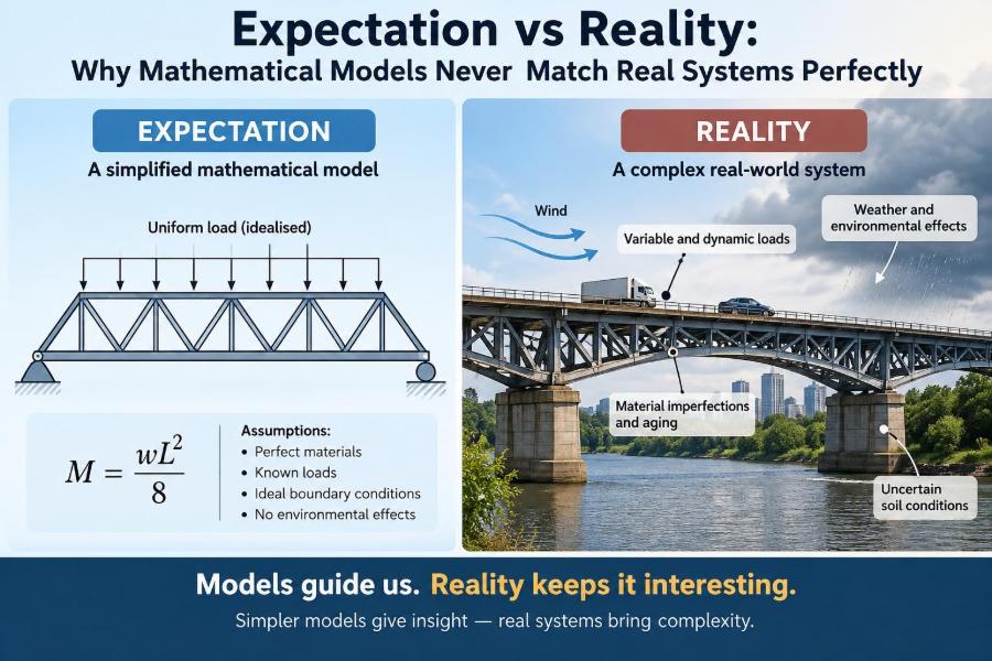

A navigation app predicts that a journey will take 24 minutes. Then a delivery van stops in a narrow lane, rain slows traffic, and a roadworks signal changes the route. The prediction was not useless; it simply described a cleaner version of the journey than the one that unfolded.
The same pattern appears in engineering. A beam calculation gives a deflection, a control model predicts a motor speed, and a heat-transfer equation estimates how quickly a tank cools. Measurements arrive, and the real system is a little different—sometimes harmlessly so, sometimes enough to matter.
This gap can feel like a failure of mathematics. It is usually better understood as a feature of modelling. A model is not the physical system; it is a deliberately limited representation built to answer a particular question.
Learning to work with that limitation is one of the most practical parts of engineering mathematics. It helps us make predictions honestly, design with margin, detect trouble early, and know when a neat equation needs to give way to new evidence.
🗺️ A Model Is a Purposeful Map, Not the Territory
A mathematical model converts aspects of a real system into variables, equations, rules, and assumptions. For a falling object, that might mean mass, gravity, and air resistance. For a production line, it could mean processing times, arrival rates, and machine availability.
Like a map, a model leaves things out on purpose. A road map does not show every tree or pavement crack because those details usually do not help someone navigate. The useful question is not whether a model includes everything, but whether it includes what matters for the decision at hand.
🎯 Every Model Begins with a Question
There is no universally “correct” model of a system. There are models that are fit for particular purposes. A building-energy model used to compare insulation options can be much simpler than one used to tune real-time heating controls.
Before writing equations, define the output that matters: maximum stress, average waiting time, fuel use, temperature range, failure probability, or something else. This choice determines which mechanisms deserve detail and which can reasonably be approximated.
✂️ Simplification Is Not Carelessness
Engineers often assume uniform material properties, rigid supports, smooth surfaces, constant flow rates, or perfectly mixed fluids. These assumptions make a problem solvable and its results interpretable.
The mistake is not simplifying. The mistake is treating an assumption as an observed fact. A useful model records its assumptions clearly, so a user can judge whether they remain reasonable in the situation being analysed.
🔍 The First Source of Mismatch: Missing Variables
Real systems contain more influences than a practical model can represent. Wind direction may affect a drone; operator behaviour may affect a plant; a supplier’s delay may affect inventory. If an omitted influence has a meaningful effect, the model may show a systematic gap from reality.
Adding variables is not automatically the cure. Each new variable needs data, parameters, and a defensible relationship to the output. Extra detail can create a model that is harder to use without making its predictions better.
📏 Parameters Are Estimated, Not Revealed Perfectly
Many equations contain parameters: friction coefficients, spring constants, reaction rates, demand elasticities, or thermal conductivities. In principle, a parameter represents a property of the system. In practice, it is often estimated from tests, manufacturer data, or historical measurements.
Those estimates have uncertainty. They may also change with temperature, age, loading, moisture, or operating condition. A model can have an excellent structure and still predict poorly because one influential parameter is slightly wrong.
🌡️ Real Properties Often Change with Conditions
Textbook problems commonly use constant values because they expose the main mathematical behaviour. Yet viscosity changes with temperature, battery performance changes with state of charge, and material stiffness can depend on temperature and load history.
A constant-property model may still be appropriate over a narrow operating range. It becomes risky when the system travels far beyond that range. The relevant issue is the size of the resulting output error, not the mere fact that a property varies.
🎲 Randomness Is Part of Many Systems
Some differences are not caused by a flawed equation. They are inherently variable. Customer arrivals fluctuate, manufacturing dimensions scatter, wind gusts change, and electronic signals contain noise.
A deterministic model gives one output for one input. A probabilistic model describes a distribution of possible outputs. When variability drives the decision, reporting only a single “expected” value can hide the risk that a less common but costly outcome will occur.
📊 Expectation Is an Average, Not a Promise
In probability, an expectation is a weighted average over possible outcomes. If a queue is expected to have ten people, that does not mean it will always have exactly ten, or even that ten is the most frequent observation.
This distinction matters in design. Average rainfall does not describe a storm drain’s peak demand, and average electrical load does not necessarily determine a cable’s required capacity. Engineers must ask whether the mean, the extremes, or the full spread is the quantity that governs safety and performance.
🧪 Measurement Data Have Limits Too
Reality is not observed directly without error. Sensors have resolution limits, calibration drift, delay, bias, and noise. Data may be missing during precisely the conditions that are hardest to measure.
If a temperature sensor reads consistently high, fitting a model to its readings can create an apparently accurate but biased model. Comparing predictions with measurements requires attention to the quality of both, not just the equation.
🕒 Time Delays Can Change System Behaviour
A model may assume that a control action immediately affects the output. Physical systems rarely behave that way. Heat takes time to travel, fluids take time to move through pipes, and information takes time to reach a controller.
Ignoring delay can be especially damaging in feedback systems. A controller that corrects an old condition may overreact, causing oscillation or instability. A simple delay term can be more valuable than several decorative details elsewhere in the model.
🔄 Feedback Makes Cause and Effect Less Obvious
In an open-loop calculation, an input produces an output. In a feedback loop, the output changes future inputs. A thermostat reads room temperature and changes heating, which then changes room temperature again.
Feedback can stabilise a process, but it can also amplify errors. Demand forecasts affect stock orders; stock availability affects sales; sales data then feed the next forecast. Models of feedback systems need to represent these loops rather than assume that each cause acts only once.
🧩 Interactions Create Effects That Single Factors Do Not
Factors often interact. High temperature and high humidity may together affect equipment differently than either condition alone. A crack and repeated vibration can cause damage that neither feature would predict independently.
Models frequently approximate a total effect by adding separate contributions. That works only when interactions are weak or unimportant for the chosen output. Where interaction is central, experiments or more detailed physics may be needed to identify it.
🏭 Boundary Conditions Are Rarely Perfect
Equations need boundary conditions: a fixed temperature at a wall, a known force at a support, a specified inlet velocity, or a defined voltage. These are essential because they anchor the mathematical solution.
Physical boundaries are more complicated. A “fixed” support may move slightly, an inlet flow may pulsate, and a wall may exchange heat with changing surroundings. Boundary-condition errors can dominate an otherwise sophisticated model.
🧱 Initial Conditions Can Be Uncertain
For time-dependent models, the starting state matters. A chemical reactor may not be fully mixed at the moment a run begins; a battery may have uncertain internal temperature; a machine may start with residual vibration.
If the system is stable and operated for a long time, it may eventually forget small initial differences. During start-up, emergency response, or short-duration processes, however, initial uncertainty can strongly shape the outcome.
📐 Discretisation Replaces Continuity with Steps
Many engineering models are solved numerically. A continuous beam becomes a finite set of elements; a fluid domain becomes a mesh of cells; time becomes a sequence of time steps. This process is called discretisation.
It makes complex problems computable, but it introduces approximation error. A mesh that is too coarse may miss a sharp stress concentration, while a time step that is too large may overlook rapid dynamics. Numerical answers should be checked for sensitivity to these choices.
💻 Computation Can Be Precise Without Being Accurate
A simulation may return six decimal places. Those digits indicate how precisely the program completed its arithmetic, not how closely the answer matches the physical world.
This is a crucial distinction. Precision describes repeatability or numerical detail; accuracy describes closeness to reality. A highly precise result based on uncertain inputs and weak assumptions should not be presented with unjustified confidence.
📉 Calibration Can Improve Fit—and Conceal Problems
Calibration adjusts parameter values so a model agrees with observed data. It is often necessary and useful. For example, a thermal model may need measured heat-loss data to estimate an effective heat-transfer coefficient.
But calibration can compensate for missing physics. A wrong parameter may be adjusted until the model matches one dataset, then fail under new conditions. A good calibration process uses physically plausible parameter ranges and tests the model beyond the data used to tune it.
✅ Validation Tests the Model Where It Must Work
Verification asks whether the equations were solved correctly: was the code implemented properly, and does the numerical method converge? Validation asks a different question: does the model represent the real system well enough for its intended use?
Validation compares predictions with independent observations where possible. “Independent” matters: using the same data to build and judge a model makes success look easier than it really is. A model that fits past data is not automatically reliable in future conditions.
🧭 Extrapolation Is More Dangerous Than Interpolation
Interpolation estimates behaviour between conditions already represented in the data. Extrapolation predicts beyond them. A model fitted to moderate loads, for example, may be asked to predict behaviour at much higher loads where a new failure mechanism appears.
Extrapolation is sometimes unavoidable, especially in early design. It should be labelled as such and accompanied by stronger margins, scenario analysis, or targeted testing. Familiar equations do not remove the risk of entering an unfamiliar regime.
⚖️ Model Complexity Has a Cost
More detailed models can capture more mechanisms, but they need more inputs, more calibration, more computation, and more opportunities for error. They can also become difficult for colleagues to inspect and challenge.
| Model choice | Strength | Common limitation |
|---|---|---|
| Simple analytical model | Fast, transparent, useful for first estimates | May omit local or nonlinear effects |
| Detailed numerical model | Can represent geometry and coupled mechanisms | Needs reliable inputs and verification |
| Data-driven model | Can detect patterns in measured data | May fail when conditions differ from training data |
| Hybrid model | Combines physical structure with data correction | Requires careful integration and interpretation |
The best choice is often the simplest model that is adequate for the decision, with its uncertainty made visible.
🧠 Data-Driven Models Do Not Escape Reality
Machine-learning models can find complicated patterns without explicitly writing every physical relationship. This is valuable for forecasting, fault detection, and surrogate modelling, where a fast approximation stands in for an expensive simulation.
They still depend on data quality, representative operating conditions, and sensible targets. A pattern learned from routine operation may not describe rare failures, new equipment, or a changed environment. Physics-based constraints can help keep predictions plausible when data are limited.
🌊 Nonlinearity Can Produce Surprising Changes
A linear model assumes that doubling an input doubles its effect, or that separate effects simply add. Many systems are nonlinear: aerodynamic drag rises strongly with speed, friction may change with motion, and a component can suddenly buckle after a threshold is crossed.
Nonlinear systems may behave calmly in one region and very differently in another. A model that works near a nominal operating point can therefore be misleading during overload, saturation, start-up, or failure conditions.
⚠️ Rare Events Can Matter More Than Typical Ones
Routine data mostly describe routine conditions. Yet engineering decisions often concern events that are infrequent but consequential: extreme loads, power interruptions, unusual combinations of faults, or operation near physical limits.
It is rarely possible to model every rare event in full detail. The practical response is to identify credible scenarios, understand the consequences, and apply safeguards. Safety factors, redundancy, containment, and operating limits are ways of managing uncertainty rather than pretending it is absent.
🛡️ Safety Margins Are Not Admissions of Defeat
A factor of safety or design margin provides room for uncertainty in loads, material properties, modelling assumptions, manufacturing variation, and future degradation. It is an engineering judgement informed by the consequences of failure and the confidence in available knowledge.
A margin should not become a substitute for understanding. If a model misses an important failure mode, multiplying its result may not fix the problem. Margins work best when paired with clear assumptions, inspection plans, testing, and conservative operating rules.
🔧 Sensitivity Analysis Finds What Actually Matters
Sensitivity analysis changes inputs or assumptions and observes how much the output moves. If a small uncertainty in one parameter produces a large output change, that parameter deserves closer measurement or a more cautious design.
This method prevents teams from spending equal effort on every unknown. For a pump system, uncertainty in pipe roughness may barely affect one design but dominate another operating range. Sensitivity turns “we are unsure” into a ranked list of priorities.
📦 Scenario Analysis Tells a More Honest Story
A single forecast suggests a single future. Scenario analysis examines several plausible combinations of conditions: low, nominal, and high demand; hot and cold ambient temperatures; new and degraded components.
Scenarios do not predict every outcome. They reveal whether a design is robust or fragile. When a conclusion holds across reasonable scenarios, confidence increases; when it changes sharply, the decision may need more data, a different design, or explicit contingency plans.
🔁 Update Models as Systems Change
Models age. Equipment wears, software updates alter control logic, users change behaviour, and construction changes the environment around a system. A once-valid model can drift away from reality without any mathematical error in its original formulation.
Operational models should have a review path: compare predictions with measurements, investigate persistent residuals, recalibrate when justified, and document what changed. This is especially important when a model supports maintenance, safety, or repeated high-value decisions.
🗣️ Communicating Uncertainty Is Part of the Engineering Work
Decision-makers may prefer a definite number, but a naked number can be misleading. Engineers should state the predicted range where possible, the main assumptions, and the conditions under which the result applies.
Clear communication does not mean burying people in caveats. It means distinguishing a robust conclusion from a tentative estimate. For example: “The design meets the target under the tested load range; behaviour above that range has not been validated.”
🚫 Common Ways Modellers Mislead Themselves
Many modelling failures begin with reasonable work interpreted too confidently. Watch for these recurring traps:
- Confusing a good fit with a good explanation: several wrong models can match the same limited dataset.
- Ignoring residual patterns: repeated overprediction or underprediction often signals missing structure.
- Using nominal inputs only: typical conditions may not govern the design.
- Reporting false precision: extra decimal places do not reduce uncertainty.
- Reusing a model outside its range: a validated model has boundaries as well as strengths.
🧰 A Practical Workflow for Trustworthy Modelling
A disciplined workflow makes limitations visible early, when they are cheapest to address. The steps do not eliminate uncertainty; they make it manageable.
- Define the decision, output, operating range, and acceptable error.
- List assumptions, omitted effects, inputs, and their likely uncertainty.
- Build the simplest model that can address the question.
- Verify calculations and numerical implementation.
- Compare with suitable measurements or established benchmarks.
- Run sensitivity and scenario checks, including relevant extremes.
- Communicate limits, margins, and conditions of use.
- Update the model when evidence shows that the system has changed.
🏗️ An Example: Predicting Room Temperature
Suppose a simple model predicts the temperature of an office using outdoor temperature, heater power, wall insulation, and room volume. It may be quite effective for planning approximate heating capacity.
Reality adds open doors, sunlight through windows, occupancy, equipment heat, intermittent heating, thermal storage in furniture, changing wind, and imperfect sensor location. The model need not include every one of these effects to be useful.
If the goal is selecting a heater, an uncertainty range and conservative design condition may be enough. If the goal is controlling temperature minute by minute, delays, occupancy patterns, sensor bias, and solar gain may become essential. The required fidelity changes with the decision.
🤝 Better Models Often Come from Better Questions
When prediction and observation differ, the first response should not always be “make the model more complicated.” Ask what pattern the mismatch has. Does it happen only at high load, after long operating times, in one location, or after a particular intervention?
Those questions can identify the missing mechanism or expose a faulty measurement. They also encourage collaboration: operators, technicians, designers, and analysts often see different parts of the same system.
🌟 The Core Principle: Useful Beats Perfect
Mathematical models never match real systems perfectly because real systems are variable, partly observed, evolving, and affected by more mechanisms than any one representation can include. Equations, data, and simulations are tools for reducing uncertainty, not abolishing it.
A trustworthy model has a clear purpose, defensible assumptions, checked calculations, evidence-based validation, and openly stated limits. It is judged by whether it supports a sound decision within its intended range—not by whether it produces the most elaborate answer.
The goal of engineering mathematics is not to create a perfect copy of reality, but to build models whose imperfections are understood well enough to act wisely. 📐🔧🌍