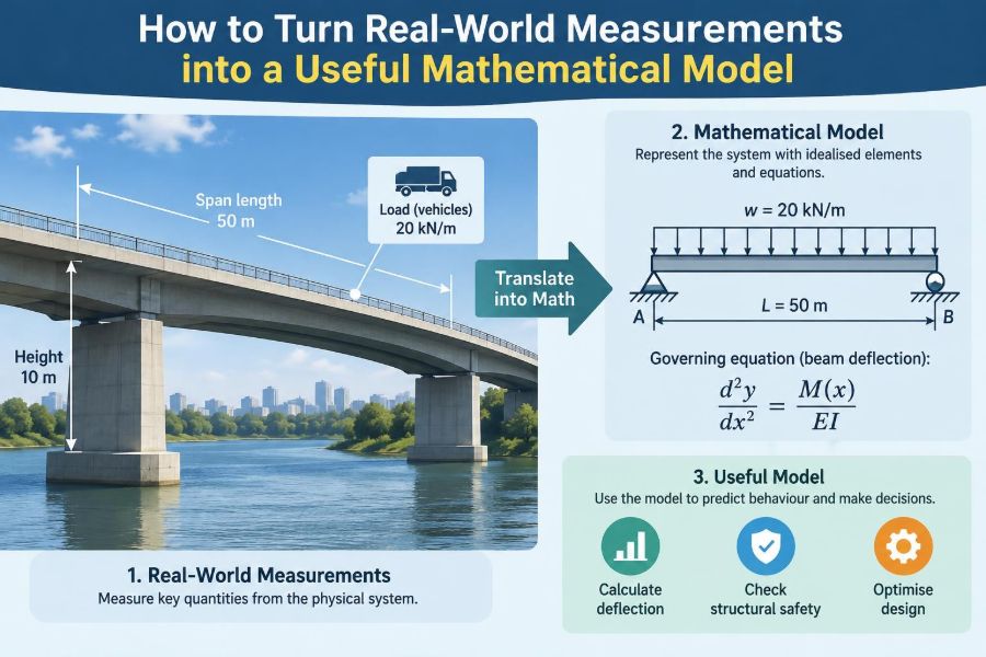

A technician records the temperature of a machine casing every minute. A civil engineer surveys ground elevations before designing drainage. A warehouse manager tracks orders, staffing, and dispatch times. Each situation begins with measurements, but measurements alone do not explain what will happen next.
The useful step is turning observations into a mathematical model: a deliberately simplified representation that connects inputs, conditions, and outcomes. A good model can estimate, compare, predict, or help make a decision without pretending to reproduce every detail of reality.
That translation is harder than it first appears. Real measurements are incomplete, noisy, rounded, and taken under changing conditions. The choice of what to include, what to ignore, and how to test the result matters as much as the equation itself.
This practical workflow applies whether you are analysing a laboratory experiment, a production process, an energy system, a transport route, or an everyday problem such as estimating water use at home.
🧭 Start with a decision, not an equation
A model should be built to serve a defined purpose. “Model the system” is too broad; “estimate next week’s electricity demand under typical weather” gives the work a direction.
Your purpose determines the acceptable error, the time horizon, and the variables that matter. A model for quick operational scheduling may be simple and updated often, while a safety-critical design model may need a larger margin and more careful validation.
- Prediction: What is likely to happen under stated conditions?
- Estimation: What quantity cannot be measured directly?
- Design: What dimensions or settings meet a requirement?
- Control: What input should be adjusted to achieve an output?
🎯 Define the output you actually need
The model’s output, often called the response variable or dependent variable, should be measurable or at least clearly calculable. Examples include stopping distance, tank level, heat loss rate, travel time, or product defect count.
Be specific about units and timing. “Temperature” could mean air temperature, surface temperature, maximum temperature over an hour, or average temperature over a shift. Those are different quantities and may require different models.
A sharply defined output prevents a common failure: collecting interesting data that cannot answer the practical question.
🔍 Draw the system boundary
Every model has a boundary. Inside it are the components and processes you intend to represent; outside it are influences treated as fixed, negligible, or separately specified.
For example, a simple model of water cooling in a cup might include the water, cup, and surrounding air temperature. It might exclude small air currents, evaporation, and changes in room temperature over a few minutes. That can be reasonable for one purpose and unacceptable for another.
Writing down the boundary exposes assumptions before they become hidden errors.
📦 Identify inputs, outputs, states, and parameters
These four categories make a messy physical situation easier to organise. They also stop us from treating every measured number as the same kind of quantity.
| Category | Meaning | Example in a heated room |
|---|---|---|
| Input | A quantity applied to the system | Heater power setting |
| Output | A quantity the model predicts or explains | Indoor air temperature |
| State | A condition that changes over time | Current room temperature |
| Parameter | A characteristic treated as fixed in one model run | Effective heat-loss coefficient |
A parameter may not truly be constant forever. It is simply stable enough over the model’s intended conditions to be represented by one value.
📏 Choose measurements that connect to the mechanism
Measure variables with a plausible relationship to the output. If you are estimating pumping energy, flow rate, pressure difference, operating time, and pump efficiency may be relevant. The colour of the pipe probably is not.
This does not mean every causal factor must be measured. Some can be controlled, held approximately constant, or represented through an uncertainty range. The point is to collect data that can distinguish between credible explanations.
Use domain knowledge first. A large spreadsheet cannot compensate for measuring the wrong physical quantities.
🧮 Establish consistent units
Unit consistency is one of the simplest and strongest checks in engineering mathematics. If a calculation combines metres, millimetres, seconds, and hours without explicit conversion, the numerical answer may look plausible while being wrong by a large factor.
Choose a unit convention early, commonly SI units for technical work, and convert raw measurements before fitting equations. Keep original records too, so conversions can be checked.
Dimensional analysis asks whether the units on both sides of an equation match. For instance, distance equals speed multiplied by time because units of metres per second times seconds reduce to metres.
🗂️ Record context alongside each measurement
A data point without context is often less useful than it looks. Record when and where it was taken, which instrument was used, operating conditions, calibration status, and any unusual events.
Imagine repeated vibration measurements on a motor. A higher reading could reflect a genuine fault, a different mounting position, a changed speed, or a sensor that was not seated properly. Context helps separate process changes from measurement changes.
Good records also make a model reproducible. Someone else should be able to understand what a column means without relying on memory.
🧪 Understand accuracy, precision, and resolution
Accuracy is closeness to the true value. Precision is the consistency of repeated measurements. Resolution is the smallest displayed or detectable increment. They are related but not interchangeable.
A scale that consistently reads 0.2 kg too high can be precise but inaccurate. A temperature display with 0.1°C increments has fine resolution, but that alone does not show that its readings are accurate to 0.1°C.
Match instrument capability to the decision. There is little value in reporting many decimal places when the sensor, procedure, or system variation cannot support them.
📉 Look at the raw data before fitting anything
Plot measurements before choosing a formula. A scatter plot can reveal a linear trend, a curved relationship, a threshold, a repeated cycle, a sudden regime change, or a recording mistake.
For data measured over time, graph the value against time. For one variable influencing another, graph output against input. A simple plot often identifies patterns that are invisible in a table.
Also inspect the spread. Two systems can have the same average output but very different variability, which changes how confidently the model can be used.
🧹 Clean data without erasing inconvenient evidence
Data cleaning means correcting known transcription problems, standardising formats, documenting missing values, and investigating unusual observations. It does not mean deleting points merely because they do not fit the hoped-for equation.
An outlier may be caused by a sensor error, but it may also reveal a different operating condition, an intermittent fault, or a limitation in the model. Keep a log of what was changed and why.
- Check impossible values, such as negative elapsed time.
- Check duplicated records and inconsistent time stamps.
- Flag missing data rather than quietly replacing it.
- Verify suspect readings against notes, instruments, or repeat measurements where possible.
🔗 Use plots to suggest a relationship, not to prove one
If two variables rise together, they are associated in the available data. That does not automatically show that one causes the other. A third variable may affect both.
For example, electricity demand and ice-cream sales could both increase during warm weather. A model intended to predict demand may still use temperature effectively, but it should not claim that ice-cream sales physically cause electricity use.
Mechanism matters. Combine observed patterns with physical reasoning, process knowledge, and controlled comparisons when available.
📈 Start with the simplest defensible model
A simple model is easier to interpret, test, communicate, and maintain. Begin with the simplest relationship that matches the purpose and does not contradict known behaviour.
A straight-line model has the form y = mx + b, where m describes the rate of change and b is the value predicted when x = 0. It is often useful over a limited range, even when the full physical relationship is more complicated.
Simplicity is not the same as naivety. A model should include enough structure to represent the dominant effects within its stated range.
📐 Let physical principles guide the equation
Whenever possible, build on conservation laws and established mechanisms. Conservation of mass, energy, momentum, and electrical charge provide powerful starting points because they constrain what an equation can reasonably do.
For a tank, a basic mass balance says that the change in stored liquid equals inflow minus outflow. For a resistor, electrical power can be related to voltage and current. These relationships give models a physical foundation instead of relying solely on curve fitting.
Measured data then helps estimate unknown parameters, assess approximations, and reveal where the idealised equation stops working.
🧠 Recognise common model families
Different patterns call for different mathematical forms. Selecting a family is a hypothesis about the system, not a final answer.
Useful starting forms
- Linear: constant change in output per unit change in input.
- Polynomial: smooth curvature over a limited interval; higher orders require caution.
- Exponential: growth or decay proportional to the current amount, such as idealised cooling or radioactive decay.
- Periodic: repeating behaviour, such as seasonal or rotating-machine effects.
- Piecewise: different equations in different operating regions, such as a valve that opens only above a threshold.
- Dynamic differential equation: output depends on its current state and rate of change over time.
The best form is the one that is credible, adequately accurate, and usable for the intended decision.
🧷 State assumptions in plain language
Assumptions turn an unmanageable reality into a solvable problem. They should be visible, testable, and connected to conditions where they may fail.
For a hypothetical falling-object model, you might assume constant gravitational acceleration, negligible air resistance, and motion in one vertical direction. Those assumptions can produce a useful first estimate, but they are poor for a light object moving fast through air.
Stating assumptions does not weaken a model. It tells users how to apply it responsibly.
⚙️ Estimate unknown parameters from measurements
Many equations contain parameters that cannot be read directly from a specification sheet. Calibration or parameter estimation uses observed data to choose parameter values that make model predictions reasonably match measurements.
In a linear model, a fitted line can estimate slope and intercept. In a heat-loss model, experimental cooling data may help estimate an effective heat-transfer parameter. Software can perform the calculations, but you still need to decide whether the result makes physical sense.
A parameter with an implausible sign, magnitude, or unit may signal poor data, a wrong model form, or a parameter that is trying to compensate for a missing variable.
🧩 Avoid fitting more flexibility than the data supports
A highly flexible equation can trace historical data extremely closely while performing poorly on new cases. This is overfitting: the model has learned random variation or accidental features rather than the underlying relationship.
Warning signs include large swings between nearby points, parameters with no interpretable meaning, and excellent fit on one dataset followed by poor predictions elsewhere.
Prefer a modest model unless extra complexity gives a clear improvement on independent data and can be justified by the system mechanism.
🧾 Calculate residuals to see what the model misses
A residual is the difference between a measured value and the corresponding model prediction. Residuals are not just errors to minimise; their pattern contains diagnostic information.
If residuals are scattered randomly around zero with no obvious trend, the model may be capturing the main structure. If they curve systematically, widen as the input increases, or cluster by operating condition, the model is missing something.
For example, a straight line may underestimate at both low and high flow rates while overestimating in the middle. That pattern suggests curvature, not merely random noise.
🧪 Separate calibration data from test data
Testing a model on the same data used to tune it can make performance appear better than it really is. When sufficient data is available, reserve some observations for validation.
One practical approach is to fit the model using one set of runs and evaluate it on later runs taken under comparable conditions. For time-dependent systems, preserve time order; randomly mixing future and past records can create an unrealistically easy test.
Validation is strongest when the test conditions resemble intended use while still including ordinary variation.
✅ Validate against the real purpose
A model can have a low average numerical error and still be unsuitable. It may miss peak loads, predict the wrong direction after a control change, or fail precisely in the operating range that matters.
Define success criteria before validation. A preliminary sizing calculation may need correct order of magnitude. A manufacturing control model may need reliably bounded error near a quality limit. A safety-related application may require formal procedures, independent review, and conservative treatment of uncertainty.
Accuracy is meaningful only relative to a decision and its consequences.
🌫️ Represent uncertainty rather than hiding it
Every model result has uncertainty from measurements, assumptions, simplified physics, natural variation, and future conditions. Reporting a single number without context can imply more confidence than the evidence supports.
Depending on the task, uncertainty can be communicated as a plausible range, an interval based on a stated method, several scenarios, or a sensitivity analysis. The method should match the data quality and the importance of the decision.
Do not turn uncertain inputs into falsely precise outputs. More digits from a calculator do not create more knowledge.
🎛️ Use sensitivity analysis to find what matters most
Sensitivity analysis changes one input or parameter at a time, or varies several systematically, to see how much the output changes. It identifies where better measurements or tighter process control would have the greatest value.
Suppose a model estimates daily energy use from occupancy, outdoor temperature, equipment power, and operating hours. If small changes in operating hours shift the result far more than reasonable uncertainty in the other inputs, effort should focus on recording hours accurately.
This is also a check on fragility. A model that changes dramatically after a tiny, plausible input change deserves close inspection.
🗺️ Respect the model’s valid range
A relationship observed in one range should not automatically be extended beyond it. Using a fitted line outside the measurements is called extrapolation, and it is generally riskier than interpolation within the observed range.
A battery discharge model fitted at moderate temperatures may be unreliable in extreme cold. A production-rate model based on normal staffing may fail during a major shift change or equipment outage.
State valid ranges for inputs, operating conditions, and time horizons. If extrapolation is unavoidable, label it clearly and use wider uncertainty bounds.
⏱️ Account for time delays and changing conditions
Many real systems do not respond immediately. A thermostat changes heater input now, but room temperature changes gradually. A demand forecast may depend on weather forecasts, schedules, and prior demand, not only the current reading.
Ignoring delays can create misleading causal conclusions and unstable control decisions. Time-series plots, lagged variables, and dynamic equations are useful when timing is part of the mechanism.
Also ask whether parameters drift. Wear, fouling, seasonal conditions, ageing sensors, and process changes can make an older model less representative.
🧱 Build in constraints that reality requires
Physical and operational constraints prevent mathematically convenient but impossible predictions. A tank volume cannot be negative. A valve has a maximum opening. A machine cannot produce beyond its capacity without changing operating conditions.
Constraints may be embedded in the equation, handled with piecewise logic, or checked after calculation. They are especially important when a fitted model is used for optimisation, because an optimiser will otherwise exploit unrealistic parts of the formula.
A useful model should fail visibly outside feasible conditions rather than quietly producing nonsense.
🧰 Choose tools that support checking
Spreadsheets are useful for small datasets, unit conversions, quick plots, and transparent calculations. Programming environments and specialist tools can help with larger datasets, repeated simulations, optimisation, and uncertainty analysis.
Tool choice should not obscure the mathematics. Keep formulas, assumptions, source data, and versioned model files organised so that important results can be traced and checked.
Automation reduces repetitive work, but it can repeat a mistaken conversion or formula very efficiently. Include independent checks for critical calculations.
📝 Document the model so someone else can use it
A model is not complete when the graph looks good. It needs a short technical record explaining its purpose, boundary, variables, data sources, units, equations, parameter values, assumptions, validation results, uncertainty treatment, and known limitations.
Documentation is practical, not bureaucratic. It helps future users decide whether the model applies to their case, and it lets the original builder revisit the work without reconstructing every decision.
For a reusable workplace model, add instructions for updating inputs and clear warnings about invalid ranges.
🚫 Watch for common modelling mistakes
Most poor models fail through ordinary process errors rather than advanced mathematics. Recognising them early saves time and can prevent costly decisions.
- Beginning with a favourite equation rather than a defined question.
- Mixing units or omitting units from data columns and axes.
- Assuming correlation establishes a physical cause.
- Discarding inconvenient observations without investigation.
- Using an untested model beyond the conditions represented by data.
- Reporting a prediction without its assumptions and uncertainty.
- Confusing a good historical fit with reliable future performance.
🏭 Work through a compact example: estimating tank level
Consider a hypothetical process tank. An operator wants to estimate its liquid volume during a run using level measurements. The immediate output is volume, while the measured input is liquid height.
If the tank has straight vertical sides and a constant horizontal cross-sectional area A, a first model is V = Ah, where V is volume and h is liquid height. Dimensional analysis confirms that area times length gives volume.
The model assumes the tank is level, its walls are effectively vertical in the measured region, and the level sensor reports height relative to a known reference. Measurements at several known fill levels can test the relationship and estimate any offset in the sensor reading.
If residuals become systematic near the bottom because the tank has a dished base, a piecewise model may be more appropriate: one relationship for the lower shaped region and another for the straight-sided section. The model has become more detailed only where the evidence and geometry require it.
🔄 Treat models as living engineering assets
A model should be reviewed when equipment, materials, operating procedures, sensors, or target decisions change. An equation that was valid during commissioning may need recalibration after modifications or after years of wear.
Set sensible review triggers: persistent residual patterns, repeated use outside the original range, a change in measurement method, or a decision becoming more consequential. Updating does not always mean making the model more complex; sometimes it means narrowing its approved use.
Version control, dated datasets, and documented changes make model updates auditable and reduce confusion between old and current results.
🤝 Combine mathematical results with engineering judgement
Models support decisions; they do not remove responsibility for judgement. A result may conflict with an operator’s observation, known physical limits, or a recent process change. That conflict is a reason to investigate, not automatically to trust either side.
Engineering judgement asks practical questions: Does the answer have sensible units? Does it follow known trends? Are the inputs credible? What happens if the assumptions are slightly wrong? Could the consequence of error require a more conservative choice?
The strongest practice combines measured evidence, mathematical structure, and knowledgeable review.
🧭 Follow a repeatable modelling workflow
- Define the decision and the required output.
- Set the system boundary and list relevant variables.
- Choose consistent units and a measurement plan.
- Collect data with context and check its quality.
- Plot the data and use physical reasoning to select a simple model form.
- Estimate parameters, inspect residuals, and revise only when justified.
- Validate on appropriate independent observations.
- State uncertainty, assumptions, valid range, and constraints.
- Document the model and review it when conditions change.
This workflow is iterative. Discovering a weak assumption or a missing variable is not wasted effort; it is how the model becomes more useful.
✨ The core principle: useful beats elaborate
A mathematical model is a purposeful approximation, not a miniature copy of the real world. Its value comes from answering a clearly defined question with a level of accuracy, transparency, and reliability appropriate to the consequences.
Good modelling begins with careful measurement but does not end there. It requires sound units, explicit assumptions, mechanism-aware equations, honest validation, and clear limits on what the result can claim.
When those habits are in place, even a modest equation can turn scattered real-world measurements into insight that people can test, explain, and use.
The best model is the simplest one that remains credible for the decision you need to make. Measure thoughtfully, check relentlessly, and let the real system—not the elegance of an equation—set the standard. 📐🔍⚙️