📐 Explaining Laplace Transforms: Why Engineers Use Them to Solve Dynamic Systems

A car suspension settles after a bump. A room thermostat responds when the temperature drops. A motor accelerates when voltage is applied, while a circuit capacitor gradually charges. These systems all change over time, and their behavior is rarely captured by a single static equation.

Engineers often begin with differential equations: mathematical statements involving a quantity and its rates of change. They are faithful models of physical behavior, but solving them directly can become awkward when initial conditions, sudden inputs, and interconnected components are involved.

The Laplace transform offers a useful change of viewpoint. Rather than tracking every instant in time, it translates a time-dependent problem into an algebraic one in a new variable called s.

That translation is why the method appears throughout control engineering, circuits, vibrations, signal processing, and system modeling. It does not remove the physics; it organizes the mathematics so the physics is easier to analyze and design around.

🧭 Dynamic Systems Are Systems That Remember Time

A dynamic system has an output that depends not only on its current input, but also on what happened previously. An empty tank and a nearly full tank react differently to the same inflow because their starting states differ.

Examples include mechanical mass-spring-damper systems, electrical RLC circuits, chemical processes, thermal equipment, and feedback-controlled machines. Each stores or dissipates energy, material, or heat, creating behavior that unfolds rather than appearing instantly.

📈 Why Ordinary Algebra Is Not Enough

Algebra is excellent for steady-state relationships. Ohm’s law, for example, relates voltage and current in a resistor at a given instant. But inductors and capacitors depend on changing current and voltage, introducing derivatives into circuit equations.

A second-order mass-spring-damper model may contain position, velocity, and acceleration. The corresponding equation is not solved simply by isolating one variable; it must satisfy both the governing law and the system’s initial state.

🧮 The Differential-Equation Starting Point

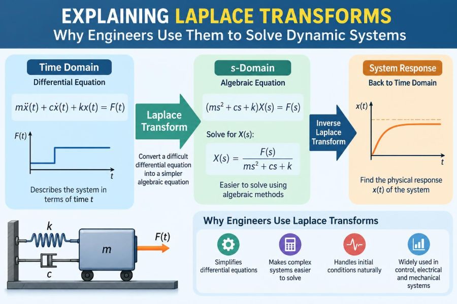
A typical linear time-invariant model can be written as a sum of derivatives of an output equaling a sum of derivatives of an input. For a mass m, damping coefficient c, spring stiffness k, displacement x(t), and applied force f(t):

m x''(t) + c x'(t) + k x(t) = f(t)

This compact equation represents Newton’s second law. Its terms respectively describe inertia, energy dissipation, restoring force, and external forcing.

🔄 The Central Idea: Change Domains

The Laplace transform maps a function of time, f(t), to a function of the complex variable s, written F(s). Formally, for suitable functions,

F(s) = ∫₀∞ e^(−st) f(t) dt

The exponential weighting makes later behavior contribute less when the real part of s is sufficiently positive. More practically, this operation turns differentiation into multiplication by s, with carefully retained information about the starting condition.

🗺️ What the s-Domain Represents

The s-domain is not merely “frequency domain,” although frequency response is closely related to it. The variable is complex: s = σ + jω. Its real part σ describes exponential growth or decay, while its imaginary part jω captures oscillation.

This makes the s-domain broad enough to represent a decaying vibration, a growing instability, a pure sinusoid, or combinations of those behaviors.

⚙️ Derivatives Become Algebraic Terms

The key operational rules are:

L{x'(t)} = sX(s) − x(0)
L{x''(t)} = s²X(s) − sx(0) − x'(0)

Instead of repeatedly integrating a differential equation, engineers work with polynomials in s. The subtracted terms are crucial: they carry the initial position, voltage, current, velocity, or other stored state into the transformed equation.

🎒 Initial Conditions Are Built Into the Method

Initial conditions describe where a system starts. A capacitor may be precharged before a switch closes; a vibrating beam may already be moving; a tank may already contain liquid.

Ignoring that stored state gives an incomplete prediction. The unilateral Laplace transform, integrating from zero onward, is especially convenient because initial values appear naturally when derivatives are transformed.

⏱️ Sudden Inputs Become Manageable

Many engineering inputs begin abruptly: a motor is switched on, a valve opens, or a force is applied at a chosen time. The unit step function models a signal that changes from zero to one at a specified time.

In the s-domain, a unit step beginning at time zero has transform 1/s. A delayed step gains an exponential factor, e^−as/s, which records the delay without forcing a separate time-domain solution for every interval.

⚡ Impulses Model Very Short Events

An ideal impulse, represented by the Dirac delta function, has zero duration but finite area. It is an approximation for a sharply concentrated event, such as a hammer tap on a structure or a brief electrical pulse.

Its transform is simply 1. This is mathematically useful because an impulse response reveals how a linear system reacts to a fundamental, highly localized input. Real impacts are never perfectly instantaneous, so the idealization must be interpreted with engineering judgment.

🧱 Standard Transform Pairs Save Time

Transform tables act like a vocabulary. Common time functions have standard s-domain forms:

Time-domain function	Laplace transform
1	1/s
eat	1/(s − a)
sin(ωt)	ω/(s² + ω²)
cos(ωt)	s/(s² + ω²)
t	1/s²

Memorizing a small core set is useful, but recognizing structure matters more. Shifts, scaling, derivatives, and products with exponentials let engineers build many transforms from familiar pairs.

🧩 Inverse Transforms Return the Physical Answer

A solved expression X(s) is not usually the final engineering result. Displacement, voltage, temperature, and current are interpreted in time, so the result must be converted back using the inverse Laplace transform.

For rational functions, partial-fraction decomposition is a common route. It separates a complicated fraction into recognizable pieces that correspond to exponentials, sinusoids, and polynomial terms in time.

🧷 Partial Fractions Expose Individual Modes

Suppose an expression contains factors such as (s+2)(s+5). Decomposition can produce terms proportional to 1/(s+2) and 1/(s+5), which invert to decaying exponentials e^−2t and e^−5t.

Those terms are not just algebraic fragments. They reveal distinct response modes, each with its own decay rate. The slower-decaying mode often dominates what remains after the initial transient has faded.

🪨 Example: A Mass, Spring, and Damper

Consider a hypothetical mass-spring-damper system initially at rest, driven by a force f(t). Transforming its equation gives:

(ms² + cs + k)X(s) = F(s)

Therefore, X(s) = F(s)/(ms² + cs + k). The differential equation has become a multiplication-and-division problem. The denominator contains the system’s inherent dynamics; the numerator describes the applied force.

🔌 Example: A Series RLC Circuit

A series RLC circuit has resistance, inductance, and capacitance, so it stores and dissipates electrical energy in a way closely analogous to the mechanical example. Depending on the selected input and output, its transformed equations also contain a quadratic polynomial in s.

This parallel is valuable. Mechanical and electrical systems may use different units and components, yet Laplace methods reveal the same underlying forms: second-order dynamics, damping, resonance, and initial stored energy.

🌡️ Example: Thermal Systems Usually Respond Slowly

A simple heated object can often be modeled by thermal capacitance, representing stored heat, and thermal resistance, representing opposition to heat flow. Its temperature does not jump immediately after heater power changes.

Many such models are first order and produce an exponential approach to a new temperature. Laplace analysis helps quantify the response rate and evaluate whether a controller will regulate temperature smoothly or react too aggressively.

🏷️ Transfer Functions Describe Input-to-Output Behavior

With all initial conditions set to zero, the ratio of output transform to input transform is the transfer function:

G(s) = Y(s) / U(s)

This is not a complete description of every possible system state; it deliberately describes the input-output dynamics under zero initial conditions. That convention makes components easier to connect, compare, and place inside larger block diagrams.

🧱 Block Diagrams Make Interconnections Visible

In a block diagram, each block represents a transfer function. Series blocks multiply, while parallel paths add. Feedback loops can also be reduced algebraically under appropriate assumptions.

For negative feedback with forward path G(s) and feedback path H(s), the closed-loop transfer function is:

G(s) / [1 + G(s)H(s)]

This form immediately shows why loop design matters: the denominator determines the closed-loop modes and therefore the response.

📍 Poles Tell You About Natural Behavior

Poles are values of s that make a transfer function’s denominator zero. They are central because they correspond to the system’s natural modes: behavior that can occur even without a continuing input.

A pole at s = −3 gives a term involving e^−3t, which decays. Complex-conjugate poles can produce decaying or growing oscillations. Pole locations are often more revealing than a lengthy inverse-transform expression.

⭕ Zeros Shape What Inputs Can Produce

Zeros are values of s that make the numerator zero. They do not usually determine stability alone, but they strongly shape transient response and frequency behavior.

A zero can attenuate certain dynamics, alter phase, or create an initially counterintuitive response in some systems. Treating zeros as unimportant because poles receive more attention is a common oversimplification.

🚦 Stability Has a Clear s-Plane Interpretation

For continuous-time linear systems, poles in the left half of the s-plane have negative real parts and correspond to decaying natural responses. Poles in the right half-plane correspond to growing responses and indicate instability in the usual input-output sense.

Poles exactly on the imaginary axis require care. An ideal undamped sinusoid may persist without growing, but small modeling changes, nonlinearities, or disturbances can matter substantially. Marginal cases are not automatically safe designs.

🎵 Frequency Response Comes From a Special Substitution

To examine sinusoidal steady-state behavior, engineers evaluate a transfer function along s = jω, where ω is angular frequency. The result describes gain and phase shift as frequency changes.

This is the mathematical basis for Bode plots and related frequency-response tools. It connects a model’s transient dynamics to practical questions: which vibration frequencies are amplified, and how much delay does a control loop introduce?

📉 Transient and Steady-State Responses Are Different

The transient response is the temporary behavior following a change, such as overshoot after a command step. The steady-state response is what remains after stable transient modes have decayed.

Laplace solutions commonly contain both. A stable system can still have unacceptable transients if it oscillates too long, overshoots a safe range, or responds too slowly for the application.

🎯 The Final Value Theorem Can Be Useful—With Conditions

When its conditions are satisfied, the final value theorem states:

lim t→∞ f(t) = lim s→0 sF(s)

It can quickly predict a stable system’s eventual output without fully inverting the transform. However, it must not be used blindly. If relevant poles indicate persistent oscillation or instability, a finite final value may not exist, and the theorem does not apply.

🧪 A Reliable Workflow for Solving Problems

1. Define the physical variables, input, output, parameters, and sign convention.
2. Write the governing differential equation from physical laws.
3. State initial conditions explicitly, including their units.
4. Take the Laplace transform term by term.
5. Solve algebraically for the desired transformed variable.
6. Inspect factors, poles, units, and limiting behavior before inversion.
7. Use partial fractions or a valid transform property to invert.
8. Check whether the time-domain answer satisfies physical expectations.

This sequence prevents a frequent mistake: performing flawless algebra on a model that was set up incorrectly.

🧠 Unit Checks Still Matter After Transforming

The variable s has units of inverse time. Consequently, terms such as sRC are dimensionless because resistance times capacitance has units of time. A denominator that adds incompatible units signals an error in modeling or algebra.

Unit checks are especially helpful when building transfer functions from physical components. They cannot prove every step is correct, but they often expose missing parameters and accidental scaling errors.

⚠️ Common Mistakes That Change the Answer

• Dropping initial-condition terms when transforming derivatives.
• Using a transfer function when the problem actually requires nonzero initial states.
• Confusing angular frequency ω with ordinary frequency in hertz.
• Canceling pole-zero factors without considering internal behavior or model uncertainty.
• Applying the final value theorem to an unstable or oscillatory expression.
• Forgetting that a delayed input requires a time-shift step after inversion.

Most of these errors are conceptual rather than computational. Writing assumptions beside the equations is often more valuable than moving faster through the manipulation.

🖥️ Software Helps, but It Does Not Choose the Model

Computer algebra systems, numerical tools, and control-design software can transform expressions, find poles, simulate responses, and generate plots quickly. They are excellent for checking work and exploring parameter changes.

They do not determine whether a damping force was modeled with the correct sign, whether sensor dynamics were omitted, or whether linearization is valid over the operating range. A polished plot can still be based on poor assumptions.

🧱 The Method Has Real Limits

Classical Laplace techniques are most direct for linear, time-invariant, continuous-time models with inputs and signals for which the transforms exist. Strong nonlinearities, changing parameters, saturation, switching, and spatially distributed systems may require approximation, numerical simulation, state-space methods, or other tools.

That is not a failure of Laplace transforms. It is a reminder that every mathematical representation has a domain where it is most informative.

🔗 Laplace Transforms and State-Space Models Work Together

State-space modeling uses first-order vector equations and handles multiple inputs and outputs naturally. It is often preferred for modern control design, nonlinear extensions, and numerical simulation.

Laplace transfer functions remain highly effective for single-input/single-output intuition, classical feedback analysis, and frequency-response design. For linear models, the two descriptions are connected: a transfer function can be derived from a state-space model when the input-output relationship is specified.

🛠️ Choosing Laplace Methods in Professional Practice

Use Laplace methods when you need an analytic understanding of transients, poles, zeros, stability, or feedback structure. They are particularly useful early in design, when changing a component value or gain should lead to a clear prediction about response.

Use simulation alongside them when inputs are complicated, nonlinear limits matter, or parameter uncertainty is significant. The strongest engineering workflow often combines hand analysis for insight with numerical tools for validation.

🌟 The Core Principle: Transform Complexity Into Structure

Laplace transforms do not make dynamic behavior disappear. They convert derivatives and initial-value problems into algebraic structure that engineers can inspect: denominators reveal modes, poles indicate stability tendencies, and transfer functions show how an input becomes an output.

The lasting value is therefore conceptual as well as computational. Once a dynamic model is expressed in the s-domain, questions about settling, oscillation, resonance, feedback, and design trade-offs become connected parts of the same picture.

Engineers use Laplace transforms because a carefully chosen change of domain turns time-dependent physics into a form that can be solved, interpreted, and designed with far greater clarity. 📐⚙️📈