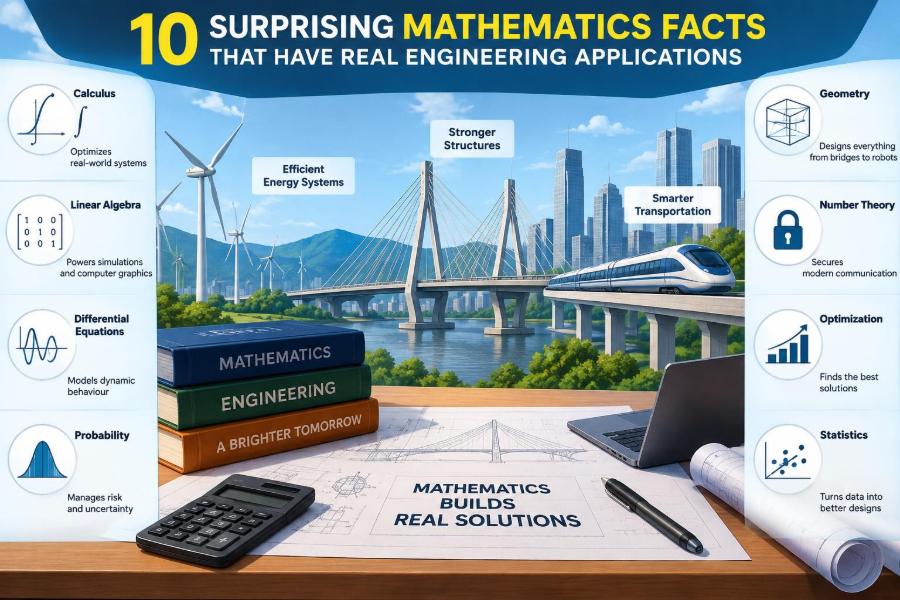

A train arrives late because a signalling system rejects noisy sensor data. A phone call stays understandable despite interference. A bridge remains steady in gusting wind instead of developing an alarming sway. These outcomes may look like separate achievements, but each depends on mathematical ideas working quietly beneath the surface.
Engineering mathematics is not only about solving textbook equations. It is a way to describe changing systems, measure uncertainty, identify hidden structure, and make defensible design decisions when materials, signals, people, and machines do not behave perfectly.
Some of its most useful ideas are also surprising. Imaginary numbers can describe real electrical power. “Holes” can reveal faults in a sensor network. Prime numbers help protect messages. Randomness can make a system more predictable.
The ten facts below connect apparently abstract mathematics to practical engineering work. The goal is not to turn every engineer into a mathematician, but to show why these tools keep appearing in designs that must be safe, efficient, reliable, and measurable.
🧭 Mathematics Is a Model, Not the Physical System
Before exploring the surprising facts, one distinction matters: an equation is a model of reality, not reality itself. A structural model might represent a building as masses, springs, and dampers; a thermal model may treat a metal plate as having a smoothly varying temperature.
Those simplifications are valuable because they isolate the behavior that matters for a decision. But every model has assumptions about geometry, material properties, loads, boundary conditions, and measurement quality.
Good engineering asks two questions at once: “Can we solve this model?” and “Is this model suitable for the situation?” A beautifully solved wrong model can produce a dangerously confident answer.
🌀 Fact 1: Imaginary Numbers Describe Very Real Oscillations
The square root of minus one, written as i, can feel disconnected from physical reality. Yet complex numbers are one of the cleanest ways to represent repeating motion, voltage, current, waves, and rotating machinery.
Euler’s relation connects exponential motion with sine and cosine:
e^(iθ) = cos(θ) + i sin(θ)
The real and imaginary parts do not imply that a voltage is “partly imaginary.” They provide a compact bookkeeping system for a quantity’s magnitude and phase—how large a wave is and where it sits in its cycle.
🔄 Phasors Turn Time-Varying Waves into Manageable Algebra
In an alternating-current circuit, voltages and currents rise and fall repeatedly. Solving directly with sine waves requires differential equations. With a complex-number representation called a phasor, engineers can often replace derivatives with multiplication by a complex frequency term.
That makes it much easier to calculate the effects of resistors, capacitors, and inductors. A capacitor and an inductor both store energy, but they shift a waveform’s timing in opposite directions; complex impedance captures that shift directly.
Once the calculation is complete, the physically measured waveform is recovered from the relevant real-valued result. The complex notation is a tool for calculation, not a claim that instruments read imaginary volts.
⚡ Complex Power Prevents Misleading Electrical Designs
Power systems use complex numbers for another reason: not all current performs useful work at every instant. Real power is converted into useful effects such as heat, light, and mechanical motion. Reactive power moves energy back and forth between sources and fields in inductive or capacitive equipment.
Motors, transformers, and transmission networks require engineers to account for both. Ignoring phase relationships can lead to undersized conductors, excessive losses, or poor voltage regulation even when a simple wattage calculation appears acceptable.
🎵 Fact 2: Any Complicated Signal Can Be Viewed as Simple Frequencies
A sharp sound, a vibration trace, or a radio transmission can look irregular in time. Fourier analysis reveals that many such signals can be described as a combination of simpler sinusoidal components at different frequencies.
This does not mean every finite real-world signal is perfectly periodic or infinitely smooth. Rather, it provides a highly useful representation: the same information can be viewed in the time domain or the frequency domain.
In the time domain, a sensor trace answers “what happened when?” In the frequency domain, it answers “which repeating rates are present, and how strongly?”
🔍 Frequency Analysis Reveals Hidden Mechanical Faults
Rotating equipment often leaves frequency signatures. A balanced fan has a characteristic rotation frequency. A worn bearing, misalignment, loose mount, or gear defect can introduce additional peaks or sidebands in measured vibration data.
Maintenance teams can compare those patterns with baseline behavior and machine speeds. The result is not an automatic diagnosis—mounting position, load, and sensor quality matter—but frequency analysis can direct inspection before a minor defect becomes a shutdown.
The same principle appears in acoustics, seismic monitoring, medical instrumentation, and structural testing.
📱 Sampling Too Slowly Creates False Signals
Digital systems do not record a continuous signal; they take samples. If the sampling rate is too low for the frequencies present, aliasing occurs. A fast variation can masquerade as a slower, false one.
The familiar visual analogy is a wheel in a film appearing to rotate slowly backward. A vibration monitor can make a similarly serious mistake if it samples too slowly and reports a frequency that was not physically present.
- Choose a sampling rate high enough for the frequency range of interest.
- Use an anti-aliasing filter before digitization to remove higher-frequency content.
- Check whether sharp transients or harmonics extend beyond the expected operating range.
📦 Fourier Methods Make Communication and Compression Practical
Frequency-based thinking also helps engineers allocate limited bandwidth. Communication systems place information into selected frequency ranges, while filters separate desired content from interference.
Compression methods often exploit the fact that some signal components matter more perceptually or contain more energy than others. An audio system, for example, can represent a signal efficiently when it understands its frequency content. The engineering trade-off is always present: stronger compression can reduce storage or transmission demand, but may introduce distortion or discard useful detail.
🏗️ Fact 3: Eigenvalues Predict the Ways Structures and Machines Want to Move
An eigenvalue is a special scaling factor associated with a transformation, and an eigenvector is a direction that keeps its direction under that transformation. That definition can sound abstract until it meets vibration.
Every flexible structure has natural patterns of motion, called mode shapes, and associated natural frequencies. In mathematical models, these emerge from an eigenvalue problem involving mass and stiffness.
A guitar string, a turbine blade, a floor slab, and a satellite panel all have modes. Their shapes differ, but the governing idea is closely related.
🌉 Resonance Is a Design Condition, Not Just a Dramatic Event
Resonance occurs when repeated forcing is near a system’s natural frequency. Energy can then accumulate, producing unexpectedly large motion. This is why engineers consider wind, rotating equipment, traffic, footsteps, engines, and earthquakes in relation to structural frequencies.
The practical response is rarely “make resonance impossible.” Instead, designers may change stiffness, mass, geometry, operating speed, or damping so that expected excitation is less troublesome.
Damping dissipates motion energy. It can be provided by material behavior, joints, fluid devices, or tuned control systems. Its effectiveness depends on the actual mode being excited, not simply on adding more material somewhere convenient.
🧪 Modal Testing Checks Whether the Mathematical Structure Matches Reality
A finite-element model may predict many natural modes, but real assemblies include bolts, welds, friction, manufacturing variation, and boundary conditions that are difficult to idealize. Modal testing measures response to controlled excitation and helps compare a model with a physical article.
Disagreement is useful evidence. It may reveal that a support is less rigid than assumed, a material property is uncertain, or a joint has been represented too simply. Engineering mathematics becomes most powerful when analysis and measurement improve each other.
🕸️ Fact 4: Networks Can Be Understood as Graphs
Graph theory represents a system as nodes connected by edges. The nodes may be intersections, servers, power substations, pipes, project tasks, or sensors. Edges represent roads, cables, transmission lines, dependencies, or communication links.
This simple abstraction ignores unnecessary visual detail and exposes connectivity: what can reach what, where bottlenecks occur, and which components are critical to the whole system.
🚰 Flow Networks Find Capacity Bottlenecks
In a flow network, each connection has a capacity. The maximum-flow problem asks how much material, information, or traffic can move from a source to a destination without exceeding those capacities.
For example, a simplified water distribution model may show that increasing pump output does little if one downstream pipe is the limiting link. In a data network, the equivalent constraint may be a congested connection rather than the processing capacity of either endpoint.
Real pipe and traffic systems have pressure losses, variable demands, and human behavior, so they need richer models. Still, network flow analysis often identifies where further investigation will be most valuable.
🛣️ Shortest Is Not Always Fastest or Safest
Shortest-path algorithms are used in routing, robotics, PCB trace layout, and logistics. But “shortest” depends entirely on what is assigned as edge cost. Distance is only one possible cost.
A route-planning model can instead penalize travel time, energy use, steep slopes, collision risk, tolls, or unreliable roads. A robot moving through a warehouse may choose a slightly longer route that preserves battery life or reduces conflict with people.
The lesson is subtle but essential: the objective function defines what the algorithm considers good. If the cost function omits a real consequence, the optimized answer may be operationally poor.
🎯 Fact 5: Optimization Finds the Best Trade-Off, Not a Magical Perfect Design
Calculus helps locate minima and maxima by examining how outputs change with inputs. Modern engineering optimization extends that idea to many variables, constraints, discrete choices, uncertainty, and competing goals.
An aircraft component might be made lighter, stiffer, cheaper, easier to manufacture, and more durable—but not all at once. Optimization formalizes the trade-off instead of leaving it entirely to intuition.
📉 Gradients Show the Direction of Fastest Change
A gradient is a vector pointing in the direction where a quantity increases most rapidly. If a design objective is mass, its gradient indicates how small changes in dimensions or materials affect mass locally.
Optimization methods use gradients, estimates of gradients, or search strategies to improve designs iteratively. They are widely used in shape design, process control, machine learning, and parameter fitting.
However, a gradient only describes nearby behavior. A nonlinear design space can contain several local minima, where a method may stop even though a better design exists elsewhere.
⚖️ Constraints Turn a Good-Looking Answer into an Engineering Answer
An unconstrained optimization might suggest an extremely thin beam because it minimizes material. A usable design must also satisfy strength, deflection, vibration, fatigue, manufacturing, inspection, cost, and safety requirements.
Constraints can be equalities, such as a required geometric relationship, or inequalities, such as a maximum stress. They can also be uncertain: a load may vary, and a material property may have scatter.
A practical optimization study should clearly state what has been optimized, which constraints are active, and which assumptions could change the result. A single “optimal” number without this context is often misleading.
🎲 Fact 6: Randomness Can Be Designed Around Rather Than Ignored
No two manufactured parts are perfectly identical. Measurements contain noise, demand changes, wind fluctuates, and components age differently. Probability provides a language for representing this variation instead of pretending that every input has one exact value.
A probability distribution does not eliminate uncertainty. It describes plausible values and their relative likelihood under stated assumptions. The quality of that description depends on data, physics, and judgment.
📏 Averages Alone Can Hide Engineering Risk
Suppose two batches of components have the same average diameter. One batch is tightly clustered; the other varies widely. Their average is identical, but their assembly behavior and likelihood of out-of-tolerance parts can be very different.
Engineers therefore inspect variation, not just mean values. Standard deviation, percentiles, tolerance limits, and worst-case bounds each answer different questions. Choosing one depends on the consequence of failure and the evidence available.
The central limit theorem helps explain why averages of many independent effects often become approximately bell-shaped. But it is not permission to assume that every dataset is normal, independent, or free of rare extremes.
🧭 Bayesian Updating Makes Sensor Data More Useful
Bayesian reasoning updates an existing estimate when new evidence arrives. In engineering terms, a system combines a prior prediction with a measurement, weighting each according to its uncertainty.
A navigation system is a familiar example. Motion models predict where a vehicle should be; GPS, wheel encoders, cameras, or inertial sensors provide imperfect observations. A filtering method can combine them to estimate position more reliably than any single source alone.
This works only as well as the uncertainty models behind it. A biased sensor, unexpected environment, or incorrect motion assumption can lead a filter to become confidently wrong.
🕳️ Fact 7: The Mathematics of Holes Can Detect Missing Coverage
Topology studies properties that remain unchanged under continuous stretching or bending, such as connectedness and the number of holes. It may seem remote from engineering until the “holes” represent gaps in coverage.
For a network of environmental sensors, communication relays, or autonomous devices, topology-inspired methods can help determine whether the devices form a connected network and whether uncovered regions may exist.
The analysis does not need an artistically perfect map of every boundary. Connectivity information—who can communicate with whom or which sensing regions overlap—can sometimes reveal global coverage problems.
📡 Sensor Networks Need Both Coverage and Connection
A sensor field can fail in two different ways. It may have good communication connectivity while leaving an area unsensed. Or it may cover the physical area well but contain isolated groups that cannot report data back to a controller.
Topology helps separate these questions. This is useful in applications such as structural health monitoring, industrial facilities, agricultural sensing, and search operations, where moving or adding devices is costly.
Real deployment still requires attention to radio obstruction, battery life, terrain, sensing range, and failures over time. Mathematical coverage is an aid to deployment decisions, not a substitute for field validation.
🌿 Fact 8: Fractal Geometry Explains Why Rough Surfaces Behave Differently
Many natural and manufactured surfaces show detail at several scales. Coastlines, porous materials, fracture surfaces, and some rough coatings cannot be described fully by one smooth length or area measurement.
Fractal geometry provides ways to describe scale-dependent complexity. A fractal dimension need not be an integer: it can express how a pattern fills space more richly than a line but less completely than a plane.
Engineers do not use fractals because every surface is a perfect mathematical fractal. They use scale-aware descriptions because roughness at small scales can influence contact, flow, wear, adhesion, and heat transfer.
🧱 Roughness Changes Contact, Friction, and Transport
Two apparently flat metal surfaces touch only at microscopic high points. Their real contact area can be much smaller than their visible area, affecting electrical contact resistance, friction, lubrication, and heat flow.
In porous media, passages at different scales influence how fluids move and how particles are trapped. A single average pore size may be insufficient when a process is sensitive to the smallest constrictions or the largest channels.
Scale-sensitive models must be matched to measurements. If the instrument cannot resolve the relevant roughness scale, an elaborate geometric model can create a false impression of accuracy.
📶 Fractal Ideas Also Appear in Compact Antennas
Some antenna geometries use repeated, folded patterns to fit a long electrical path into a limited physical area. This can support compact designs or behavior across multiple frequency bands.
The benefit is not universal. Fabrication limits, losses, bandwidth, radiation pattern, and nearby materials can outweigh geometric elegance. The useful takeaway is broader: mathematical self-similarity can inspire designs that use space differently from simple straight-line layouts.
🔐 Fact 9: Prime Numbers Help Secure Digital Engineering Systems
Number theory studies integers and their properties. It supports public-key cryptography, which allows devices to establish secure communication without first sharing a secret through a safe physical channel.
Many cryptographic systems rely on mathematical problems that are easy to perform in one direction but computationally difficult to reverse without secret information. Large primes and modular arithmetic are central to several well-known approaches.
The engineering application is everywhere: software updates, payment systems, industrial controllers, cloud services, vehicle communications, and remote access all depend on carefully implemented cryptography.
🗝️ Cryptography Depends on Implementation, Not Just Clever Mathematics
A strong algorithm can still fail through weak passwords, reused keys, flawed random-number generation, unpatched software, exposed private keys, or timing side channels. Security is a system property.
Engineers should avoid inventing custom cryptographic schemes for ordinary applications. Established protocols and reviewed libraries are generally safer choices, provided they are configured, updated, and managed correctly.
Cryptographic strength also changes over time as computing capabilities and attacks evolve. Design decisions should include key rotation, update paths, and a plan for replacing outdated methods.
🧩 Error-Correcting Codes Recover Information from Noise
Related mathematics allows a receiver to detect or correct some errors in transmitted or stored data. Error-correcting codes add structured redundancy, not merely duplicate copies.
A satellite link, Wi-Fi connection, QR code, solid-state drive, or deep-space communication system may receive incomplete or corrupted bits. The code’s structure allows the receiver to infer the most likely intended message when errors remain within its correction capability.
Redundancy costs bandwidth, storage, processing, or delay. Engineers select a code based on expected noise, latency limits, power budget, and the consequence of an uncorrected error.
🌪️ Fact 10: Deterministic Systems Can Still Become Unpredictable
Chaos theory studies systems governed by deterministic rules that can be extremely sensitive to initial conditions. Tiny differences in starting state can grow into large differences later.
This is not the same as pure randomness. A chaotic system follows rules, but long-term prediction may become impractical because no measurement has infinite precision.
Weather is a familiar example of this limitation. Engineering examples include nonlinear vibration, turbulent flows, electronic circuits, and control systems operating near unstable regimes.
🎛️ Feedback Can Stabilize a System—or Destabilize It
Feedback compares measured output with a target and adjusts the input. A thermostat, cruise controller, drone, and motor drive all use this principle.
Negative feedback usually counteracts an error, but delay, excessive gain, sensor noise, and unmodeled dynamics can create oscillation. If a controller reacts too aggressively to an outdated measurement, it can repeatedly overcorrect.
Control design therefore examines stability margins, response speed, actuator limits, and disturbance rejection together. Fast response is valuable only when it remains stable and robust.
💻 Numerical Methods Make Unsovable-by-Hand Problems Usable
Many engineering equations have no convenient closed-form solution for realistic geometry or material behavior. Numerical methods approximate them using a finite number of calculations.
Finite-element analysis divides a structure into smaller elements. Computational fluid dynamics divides a flow region into cells. Time-stepping methods simulate how a system evolves in small increments.
These methods are indispensable, but their output is an approximation. Mesh density, time-step size, convergence criteria, material models, and boundary conditions all influence the answer.
✅ Verification and Validation Are Different Checks
Verification asks whether the mathematical and numerical problem was solved correctly. This can include mesh refinement, code checks, conservation checks, and comparison with simpler cases that have known answers.
Validation asks whether the model represents the physical world well enough for its intended use. This requires comparison with relevant measurements or trusted physical evidence.
A simulation may be verified yet invalid if its assumptions do not match the real system. Conversely, a good physical concept can be obscured by a numerical setup error. Both checks matter.
🛠️ Choosing Mathematics by the Engineering Decision
Different questions call for different mathematical tools. The best method is not always the most advanced one; it is the one that resolves the decision with credible accuracy and manageable effort.
| Engineering question | Useful mathematical lens | Typical caution |
|---|---|---|
| Which vibration is growing? | Fourier analysis and modal methods | Check sampling and sensor placement |
| What is the lightest feasible design? | Constrained optimization | Include safety and manufacturing limits |
| Where can a network fail? | Graph theory and reliability models | Do not ignore shared failure causes |
| How uncertain is a prediction? | Probability and statistical inference | Question distribution assumptions |
| Can a controller remain stable? | Dynamics and control theory | Include delay and actuator saturation |
⚠️ Common Mistake: Treating a Precise Output as a Certain Answer
Engineering software can print ten decimal places, but that does not mean the physical prediction is accurate to ten decimal places. Input uncertainty, model form, and measurement limitations usually dominate long before arithmetic precision does.
Useful reporting distinguishes numerical precision from engineering confidence. Sensitivity studies can show which assumptions affect the conclusion most strongly. That information often matters more than one polished final value.
🧰 A Practical Workflow for Applying These Ideas
- Define the physical question and the decision it must support.
- Identify the dominant mechanisms: motion, flow, heat, uncertainty, connectivity, or information transfer.
- Select a model whose assumptions fit the required accuracy and available data.
- Calculate, simulate, or measure using appropriate numerical and experimental checks.
- Test sensitivity to uncertain inputs and plausible operating conditions.
- Communicate limitations alongside conclusions so decisions are made with proper context.
This workflow scales from a quick spreadsheet estimate to a major simulation campaign. The tools change; the discipline of connecting mathematics to physical evidence does not.
🌟 The Core Takeaway: Abstract Ideas Become Useful Through Interpretation
Complex numbers clarify phase, Fourier analysis exposes frequency content, eigenvalues reveal natural behavior, graphs map connections, optimization manages trade-offs, probability handles variation, topology finds coverage gaps, fractal ideas describe scale, number theory protects information, and nonlinear dynamics warns against false predictability.
None of these methods replaces engineering judgment. Their value comes from pairing mathematical structure with physical understanding, credible data, and careful attention to what a model leaves out.
The most useful engineering mathematics is not the mathematics that produces the longest calculation; it is the mathematics that helps you make a better, safer, more transparent decision. 📐⚙️🔎