
A bridge designer changes the thickness of a steel plate by a few millimetres. An automotive engineer adjusts the angle of an air duct. A process engineer raises a pump speed. Before anything is manufactured, each wants to know what will happen next: Will the bridge deflect too far? Will the engine run hotter? Will the pipe system vibrate?
The governing physics may fit on a page: forces balance, energy is conserved, fluid momentum changes according to pressure and viscosity. Yet the actual geometry, material behaviour, loads, and boundary conditions make most useful engineering problems too complicated for an exact hand calculation.
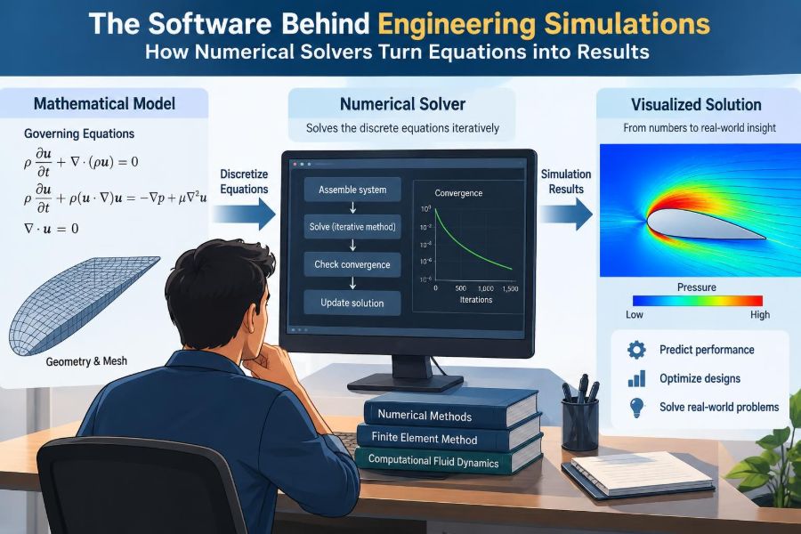
Simulation software closes that gap. It translates a mathematical model into a very large set of numerical operations, then uses a numerical solver to calculate an approximate answer that engineers can inspect, question, and improve.
Understanding that process makes simulation results more useful—and makes colourful plots much harder to trust blindly. The real skill is not merely pressing Run. It is knowing what problem the software actually solved.
🧩 A simulation is a chain, not a single calculation
Engineering simulation is often described by its final image: a stress contour, a temperature map, or streamlines around a wing. That image is the last link in a longer chain.
The chain begins with a physical question and a set of assumptions. It passes through geometry, material data, discretisation, equations, solver settings, and post-processing. A credible result requires every link to be reasonable; an excellent solver cannot repair an unsuitable model.
📜 The governing equations describe the physics
At the foundation are governing equations: mathematical statements of physical laws. Structural analysis commonly uses force equilibrium and material constitutive laws. Heat-transfer models use conservation of energy. Fluid simulations use conservation of mass, momentum, and often energy.
For example, heat conduction in a solid is governed by an equation relating temperature change to thermal conductivity and heat sources. The equation is compact, but solving it through a motor housing with bolt holes, changing materials, and convection at several surfaces is not.
🔍 Why exact analytical solutions are rare
An analytical solution is a formula that gives the answer directly, such as the familiar beam-deflection expressions taught in mechanics courses. These solutions are invaluable because they reveal physical trends and provide checks.
They usually require idealised shapes, simple loading, uniform properties, and neat boundary conditions. Real products have curved surfaces, joints, contact regions, non-uniform loads, and properties that can vary with temperature. Numerical methods trade a closed-form answer for a controlled approximation of that more realistic situation.
🧱 Discretisation breaks a continuum into manageable pieces
A solid, fluid, or thermal field is physically continuous: temperature can vary from point to point, and so can displacement or pressure. A computer cannot store infinitely many values. Discretisation replaces the continuum with a finite collection of unknowns.
In finite element analysis, or FEA, a component is divided into small elements connected at nodes. In many fluid calculations, the flow region is divided into cells called a mesh. The solver calculates values at selected locations, then uses mathematical interpolation to represent the field between them.
🕸️ The mesh sets the resolution of the question
A mesh is not just a visual grid. It determines which changes the model has enough detail to represent. A coarse mesh may capture the overall bending of a bracket while missing a sharp stress gradient around a small hole.
Very small elements are useful where gradients are steep: near contacts, cracks, boundary layers in fluid flow, heat sources, and geometric transitions. Fine resolution everywhere is rarely efficient. It increases the number of unknowns, memory demand, and solution time without necessarily improving the engineering decision.
📐 Elements and cells are mathematical approximations
Elements come in different shapes and orders. A first-order element uses a simple variation of the field within its boundaries. A higher-order element can represent curvature more smoothly, often achieving good accuracy with fewer elements in suitable problems.
No element type is universally best. Thin structures may be represented efficiently by shell elements, long members by beams, and complex three-dimensional parts by solid elements. In fluid simulations, cell quality strongly affects stability and accuracy. Distorted cells can introduce numerical error or stop a calculation from converging.
🚪 Boundary conditions make the model physically specific
Equations alone do not define a unique engineering problem. They need boundary conditions: statements about what happens at supports, surfaces, inlets, outlets, and interfaces.
A structural model might prescribe displacement at bolt locations and apply a load over a contact area. A thermal model may specify a fixed temperature, an applied heat flux, or convection to surrounding air. A fluid model may set inlet flow, outlet pressure, wall roughness, and turbulence-related quantities.
Boundary conditions are frequently the largest source of uncertainty because the real environment is often less well known than the component geometry.
🧭 Initial conditions matter when time is involved
For a steady calculation, the desired solution does not change with time. For a transient calculation, the starting state matters. A cooling casting needs an initial temperature field; a vibration model needs initial displacement or velocity; a flow start-up model needs an initial flow state.
A good initial condition can also help the solver reach a useful answer efficiently. But convenience must not become fiction. Starting a transient thermal model at room temperature is inappropriate if the real part is already hot when the event begins.
🧪 Material models determine how the model responds
Software needs a mathematical description of material behaviour. Linear elastic steel, for instance, is commonly represented with elastic modulus and Poisson’s ratio when stresses remain in the elastic range. That is a useful model, not a complete description of every steel component.
Plasticity, viscoelasticity, creep, composite anisotropy, fatigue damage, and temperature-dependent behaviour require richer models and more data. The best choice depends on the decision being made. A simple material model can be adequate for early stiffness screening but inadequate for predicting permanent deformation after overload.
⚖️ Linear and nonlinear problems behave differently
In a linear analysis, doubling the load doubles the response, the geometry is assumed not to change enough to affect equilibrium, and material properties remain in a simple range. These assumptions enable fast, robust calculations.
Nonlinear analysis is needed when contact opens or closes, deformation significantly changes the load path, materials yield, or loads themselves depend on displacement. Nonlinear models can better reflect reality, but they require careful increments, convergence controls, and interpretation. More complexity is valuable only when the underlying physical effect matters.
🔢 From equations to a system of algebra
After discretisation, the software assembles local equations from every element or cell into a large global system. In a simple structural setting, this is often represented as K u = f, where K is stiffness, u contains unknown displacements, and f contains applied forces.
Thermal and fluid systems have analogous matrices and vectors, though their terms may include diffusion, transport, pressure, velocity, or time dependence. The solver’s task is no longer to manipulate a symbolic differential equation; it is to find millions of unknown numerical values that satisfy the assembled relationships.
🧮 Direct solvers eliminate unknowns systematically
A direct solver uses matrix factorisation methods to solve the algebraic system in a systematic sequence. For a well-conditioned linear problem, it can deliver a very accurate answer relative to the discretised equations.
Its drawback is resource use. Large three-dimensional models can demand substantial memory and computation because the solver must store and manipulate large matrix structures. Direct methods are often attractive for moderate-size structural problems, multiple load cases, or cases where dependable linear-system accuracy is the priority.
🔁 Iterative solvers improve an estimate step by step
An iterative solver starts with an estimate and repeatedly improves it. Rather than fully factorising the matrix, it seeks an answer whose remaining equation error—the residual—is sufficiently small.
Iterative methods can be far more memory-efficient for very large sparse systems, which are common in computational fluid dynamics and large finite element models. Their performance depends strongly on matrix conditioning, mesh quality, scaling, and solver settings. A residual that falls slowly is not merely an inconvenience; it can indicate a modelling or numerical difficulty.
🧰 Preconditioning makes difficult systems easier to solve
Many numerical systems are awkward because some unknowns influence the equations on very different scales. Preconditioning transforms or approximates the system so that an iterative method can progress more effectively.
An analogy is arranging a cluttered workshop before beginning a repair. The task has not changed, but useful tools are now easier to reach. Preconditioners can greatly reduce iterations, although they add setup cost and may need tuning. Their details are often hidden behind software options, but their effect on run time can be dramatic.
⏱️ Time stepping turns changing behaviour into snapshots
Transient simulations advance from one time point to the next. Instead of asking only for a final temperature or displacement, they calculate a sequence of states: a brake disc heating during a stop, pressure waves moving through a pipe, or a structure responding to a shock.
The time-step size is a numerical decision with physical consequences. Large steps may miss a rapid event or smear sharp changes. Extremely small steps may make a model impractical to run. Adaptive schemes can reduce the step during difficult periods and enlarge it when the response evolves smoothly.
🌊 Stability is not the same as accuracy
A stable numerical method produces values that do not grow spuriously or oscillate without physical cause. An accurate method produces values close enough to the solution of the intended physical model. A calculation can be stable yet inaccurate if its mesh or time step is too coarse.
This distinction matters in fluid flow and transient dynamics. A simulation that finishes cleanly is not automatically trustworthy. Engineers must ask whether important length scales, time scales, and expected physical features were actually resolved.
🎯 Convergence means the numerical process has settled
For iterative and nonlinear calculations, convergence means the solver has met defined criteria. These often include small residuals, small changes between iterations, and acceptable equilibrium imbalance.
Convergence does not prove that the physical model is correct. It only says the software has found a sufficiently consistent solution to the equations, mesh, and assumptions supplied. Conversely, failure to converge may point to a real instability, but it can also arise from poor contacts, unrealistic constraints, an abrupt load application, or a low-quality mesh.
📊 Residuals, monitors, and balance checks tell different stories
A residual measures how well the current estimate satisfies an equation. It is useful, but it should not be the only progress indicator. Monitor quantities—such as drag, outlet temperature, displacement, or reaction force—show whether the engineering output has stabilised.
Balance checks provide another safeguard. In a static structural model, reactions should balance applied loads within an appropriate numerical tolerance. In a thermal model, the net energy entering and leaving should make sense. These checks connect the abstract solver process to conservation laws.
🧯 Contact is a common source of nonlinear difficulty
Contact determines whether surfaces can separate, slide, or transmit frictional force. It appears in bolted assemblies, gears, seals, press fits, and impact problems. It is physically important because the load path can change whenever a gap opens or a surface begins sliding.
Numerically, contact introduces conditional behaviour: a pair of surfaces may interact in one iteration and not in the next. Small setup choices—contact stiffness, allowed penetration, friction assumptions, and surface definitions—can strongly affect convergence and local stresses. Contact results deserve especially careful sensitivity checks.
🌬️ Fluid simulations add coupling and turbulence
In computational fluid dynamics, pressure and velocity are coupled by mass conservation. The solver must find a pressure field that makes the velocity field satisfy continuity while also solving momentum and, when needed, energy equations.
Turbulent flow adds another modelling layer. Most practical engineering simulations cannot resolve every turbulent eddy, so they use turbulence models to represent unresolved motion. Different models suit different flow features, and a result near separation, recirculation, or a wall should be interpreted with the model’s limitations in mind.
🔥 Multiphysics models connect more than one domain
Many real systems involve coupled physics. Electrical current creates heat; heat expands a structure; deformation alters contact pressure; fluid flow transports heat; magnetic forces move components. A multiphysics model connects these effects.
Coupling can be one-way or two-way. In a one-way thermal-stress study, calculated temperatures drive structural expansion, but deformation does not change the temperature field. Two-way coupling repeatedly exchanges information between domains. It is more complete when feedback matters, but it costs more and is harder to verify.
🖥️ Parallel computing makes larger models practical
Modern solvers divide work across processor cores and, in some applications, graphics processors. Different elements, cells, or matrix operations can be processed concurrently. This is why large simulations may run on workstations, clusters, or cloud infrastructure.
More processors do not guarantee proportionally faster runs. Some stages require communication or serial work, and poorly balanced partitions leave hardware waiting. Hardware can expand what is feasible, but it cannot compensate for a weak model, unsuitable mesh, or poorly chosen solver formulation.
🗺️ Post-processing turns fields into engineering evidence
The raw output of a solver is usually a large collection of numbers. Post-processing converts those values into plots, animations, paths, summaries, and derived quantities. This is where a temperature field becomes a maximum operating temperature or a displacement field becomes a clearance assessment.
Visualisation is powerful but can mislead. Colour scales can exaggerate small differences, smooth contours can hide under-resolution, and a single maximum may be a numerical singularity. Always inspect units, legend ranges, deformed-shape scale factors, and the location from which a reported value was taken.
📍 Singularities are warnings about idealisation
A stress singularity occurs when an idealised model creates an unbounded or mesh-dependent local stress, such as a perfectly sharp re-entrant corner or a point force. Refining the mesh can make the reported peak stress rise rather than settle.
This does not mean the entire model is useless. It means that one local value cannot be interpreted literally. Engineers may replace a point load with a distributed load, model the real fillet radius, examine stresses a small distance away, or use a fracture-mechanics approach when crack behaviour is the actual concern.
✅ Verification asks whether the equations were solved correctly
Verification concerns the numerical implementation: Did the mesh adequately resolve the solution? Are solver settings appropriate? Does the model reproduce a known benchmark or a simpler hand calculation?
A mesh-convergence study is a central verification tool. The analyst refines relevant regions and checks whether a target quantity, such as reaction force, pressure drop, or stress away from singularities, approaches a stable value. The goal is not the finest possible mesh; it is confidence that further refinement would not change the decision materially.
🔬 Validation asks whether the model represents reality
Validation is a different question: Does the chosen model represent the physical system well enough for its intended use? This may involve comparison with measured temperatures, test deflections, pressure data, or established experimental benchmarks.
Agreement is meaningful only when the comparison conditions match: geometry, loading, material state, sensor location, and operating conditions all matter. A simulation can be verified but invalid if its boundary condition is wrong. It can also match one test by coincidence while failing in another regime.
📏 Uncertainty should be managed, not hidden
Inputs are often uncertain. Friction coefficients vary, loads fluctuate, material properties scatter, and convection conditions are estimated rather than directly measured. Reporting many decimal places from a solver does not create corresponding physical certainty.
Sensitivity analysis explores how outputs change when plausible inputs change. For a hypothetical enclosure-cooling model, varying fan flow rate, ambient temperature, and thermal contact resistance may reveal which assumption dominates peak component temperature. That insight is often more valuable than a single nominal result.
🛠️ A disciplined simulation workflow prevents expensive errors
Reliable analysis usually follows a sequence that keeps the engineering question visible:
- Define the decision the simulation must support and the output that matters.
- Choose the simplest physics and geometry that can answer that question.
- Document loads, constraints, material data, and assumptions.
- Build and inspect the mesh, concentrating detail where gradients are expected.
- Select solver controls appropriate to linearity, time dependence, and coupling.
- Check convergence, balances, and output plausibility.
- Verify mesh and numerical sensitivity, then validate against relevant evidence where possible.
This workflow also creates traceability. Someone reviewing the result should be able to understand not only the final plot, but also why the model deserves confidence.
🚫 Common simulation mistakes have recognisable patterns
Several errors recur across disciplines. Applying a load at a single node can generate artificial peaks. Fully fixing a surface that is flexible in reality can make a part appear safer than it is. Treating uncertain contact or heat-transfer data as exact can hide the dominant risk.
- Using default solver settings without checking their assumptions.
- Judging mesh quality by appearance rather than target-output convergence.
- Reading a local peak value without examining its physical location.
- Comparing results with a test that represents different conditions.
- Adding complexity before establishing a simple, checkable baseline model.
Most of these mistakes are not software failures. They are failures to connect mathematical choices to physical meaning.
🧠 Choosing the right level of model fidelity
Fidelity is the degree to which a model represents detail in the real system. Higher fidelity can improve prediction, but it also introduces more parameters, more opportunities for incorrect assumptions, and longer turnaround time.
A preliminary design may only need beam theory and a linear FEA check. A safety-critical component near yield, with complex contact and thermal loading, may justify a nonlinear coupled model and test correlation. The appropriate model is the simplest one that is credible for the consequence of being wrong.
🤝 Engineers remain responsible for interpretation
Simulation software automates equation assembly, linear algebra, and plotting. It does not automatically decide whether an inlet condition is representative, whether a material model applies, or whether a predicted failure mode is physically plausible.
Good analysts use first-principles estimates, dimensional reasoning, hand calculations, and test observations alongside software. If a simulation predicts a result that conflicts with basic engineering intuition, the response should be investigation—not automatic rejection or unquestioning acceptance.
🏁 The core principle: solve the right approximation well
Numerical solvers are the engines inside modern engineering simulation. They turn conservation laws and constitutive relationships into calculated fields of temperature, stress, pressure, velocity, displacement, and many other quantities. Their power comes from combining mathematics with practical approximations.
The key distinction is simple: a solver can accurately solve the equations it receives, while engineering credibility depends on whether those equations, inputs, boundaries, mesh, and interpretations represent the decision at hand. Treat simulations as structured evidence, not as automatic truth.
The most useful simulation is not the one with the most detail; it is the one whose assumptions, numerical behaviour, and limits are understood well enough to support a sound engineering decision. 📐🧮🔧