
A design calculation does not become useful merely because a computer returns a number. An engineer needs to know whether that number is close enough to reality to size a beam, tune a controller, predict a pressure drop, or decide whether a simulation must run longer.
That question often appears as a progress bar, a residual plot, or a sequence of answers that changes with every iteration. One run settles in a handful of steps; another seems to improve painfully slowly; a third produces a convincing-looking answer that is wrong.
Numerical methods are the tools used when an exact analytical solution is unavailable, impractical, or too simplified for the engineering problem. Their speed of convergence determines how quickly repeated approximations approach the desired solution.
But “fast” has a precise mathematical meaning, and it is not the same as “finished,” “accurate,” or “safe.” Understanding the distinction helps engineers choose methods intelligently, set realistic stopping criteria, and avoid trusting a calculation before it has earned that trust.
🧭 What convergence means in numerical work
A numerical method creates a sequence of approximations, often written as x_0, x_1, x_2, .... It converges if those approximations approach a limiting value as the iterations continue.
For root finding, the limit may be a value of x that makes f(x)=0. In finite element analysis, it may be a displacement field. In computational fluid dynamics, it may be a stable flow solution satisfying the discretized governing equations.
Convergence is therefore about a trend. It says the method is moving toward a limit, not automatically that the limit is the correct physical answer.
🎯 The target is usually an exact solution of a model
Engineering models convert physical principles into equations: equilibrium, conservation of mass, heat transfer, constitutive behavior, and boundary conditions. A numerical method attempts to solve those equations.
This creates an important hierarchy. A calculation may converge tightly to the exact solution of the discretized model, while the model itself may omit a load case, use uncertain material data, or represent a curved geometry too coarsely.
Fast convergence is valuable, but it only reduces one part of the total uncertainty.
📏 Error is the distance from the answer you want
If the exact solution x* were known, the iteration error at step k would be e_k = x_k - x*. In real problems, however, x* is usually unknown; if it were known, there would be no need to iterate.
Engineers therefore estimate error indirectly. They inspect changes between iterates, residuals in the equations, mesh-refinement trends, benchmark cases, and physical checks such as force balance.
Keeping “error” separate from quantities that merely indicate error is one of the central habits of reliable numerical work.
🔍 Residuals measure unsatisfied equations
A residual measures how well the current approximation satisfies the equations being solved. For a scalar root problem, it is commonly r_k=f(x_k). A perfect root has zero residual.
A small residual is encouraging, but its meaning depends on scaling and conditioning. For example, a residual of one unit may be tiny for a load balance measured in meganewtons and unacceptable for a temperature requirement measured in kelvins.
In a linear system Ax=b, a small residual b-Ax does not always imply a small solution error, especially when the matrix is poorly conditioned.
⚖️ Why a small residual can still hide a large error
Suppose two nearly parallel equations intersect at a shallow angle. A small change in either equation can move the intersection a long distance. Mathematically, this is a poorly conditioned problem.
In such cases, the equations can be almost satisfied while the unknowns remain noticeably wrong. The computation has not necessarily failed; the problem itself amplifies small numerical or data errors.
This is why engineers should monitor residuals alongside solution changes, condition estimates where available, and physically meaningful output quantities.
📈 Convergence rate describes how error shrinks
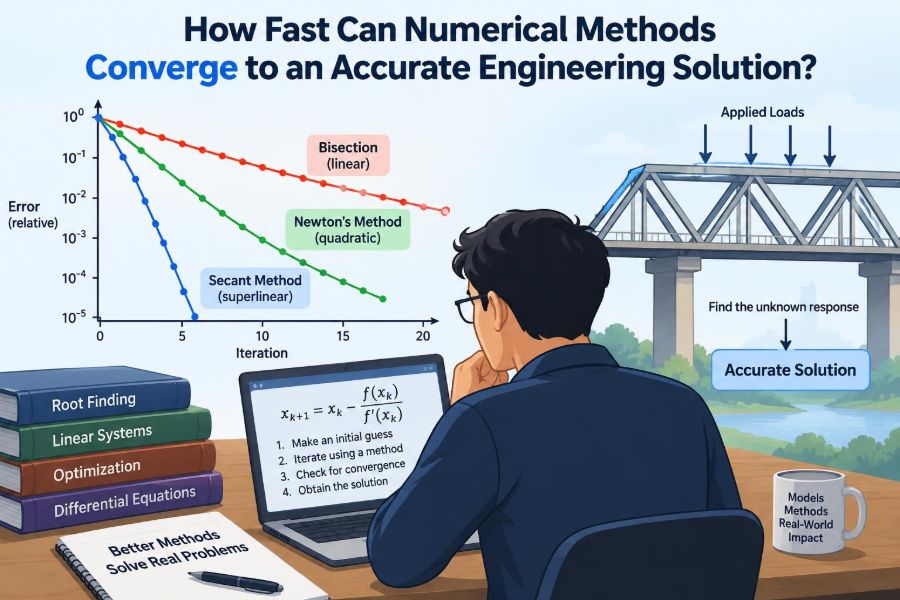
The usual local model for convergence is |e_(k+1)| ≈ C|e_k|^p, where C is a constant and p is the order of convergence.
The order describes the asymptotic behavior: what happens when iterations are already sufficiently close to the solution. It does not guarantee that the same pattern applies from a poor starting guess.
Higher order can be dramatically faster near the solution, but it may demand more work per iteration or be less forgiving when the initial estimate is poor.
🐢 Linear convergence reduces error by a factor
A method is linearly convergent when its error eventually follows approximately |e_(k+1)| ≈ q|e_k|, with 0<q<1. Each iteration removes a similar fraction of the remaining error.
If q=0.5, the error roughly halves each iteration. If q=0.95, progress is much slower: many iterations are required because only a small fraction disappears at each step.
Linear convergence is common in practical iterative solvers. It is not inferior by definition; a cheap, robust linear method can outperform a more sophisticated method with expensive or unreliable steps.
🚀 Superlinear convergence accelerates near the solution
Superlinear convergence means the error-reduction factor itself tends toward zero. The method gains efficiency as it approaches the solution, even if it does not follow one fixed integer order.
Quasi-Newton methods can show this behavior under suitable conditions. They update an approximation to derivative information rather than rebuilding an exact derivative matrix at every iteration.
This can be an excellent engineering compromise when exact derivatives are expensive but the problem is smooth enough for the approximation to improve.
⚡ Quadratic convergence can double correct digits
A quadratically convergent method has p=2. Once it reaches its local convergence region, the error is roughly proportional to the square of the previous error.
Newton’s method for a simple root is the classic example. In favorable conditions, each iteration can roughly double the number of correct digits. That is why Newton iterations can appear almost magical at the end of a calculation.
However, quadratic convergence is a local promise, not a universal one. It relies on a sufficiently good starting point, a well-behaved derivative, and a root that is not degenerate.
🧮 A root-finding example makes the contrast visible
Consider the hypothetical task of finding a pipe-flow operating point where a pump curve and system curve intersect. This can be written as a root problem, f(Q)=0, for flow rate Q.
Bisection begins with an interval known to contain a sign change. It repeatedly halves that interval. Its progress is predictable: after n steps, the interval width is the initial width divided by 2^n.
Newton’s method uses the local slope: x_(k+1)=x_k-f(x_k)/f'(x_k). Close to a simple operating point, it may reach the same tolerance in far fewer steps. But without safeguards, a poor initial flow estimate can send the iteration to an unrealistic region.
🛡️ Bisection is slow for a reason
Bisection has linear convergence, yet it is often prized because it maintains a bracket around a root when the function is continuous and the endpoint signs differ. The root cannot simply disappear from the interval.
That guarantee is useful when evaluating the function is affordable and reliability matters more than achieving the fewest iterations. It is also a dependable way to obtain a starting point for a faster local method.
Its limitation is equally clear: it uses no slope information, so it cannot exploit the smoothness of a friendly problem.
🔄 The secant method trades derivatives for speed
The secant method estimates a derivative from the two most recent points. It avoids calculating f'(x), which can be valuable when derivatives are unavailable, noisy, or costly.
For smooth scalar problems, it can converge faster than linearly and often more quickly than bisection. Yet it does not retain bisection’s bracket automatically, and its slope estimate can become poor.
A practical hybrid solver often combines bracketing logic with secant-like or inverse interpolation steps. When a fast step is unsafe, it falls back to interval reduction.
🧱 Newton’s method earns its speed with assumptions
Newton’s method requires a derivative in one dimension, or a Jacobian matrix for many variables. A Jacobian contains the local rates at which each equation changes with each unknown.
For nonlinear finite element problems, forming and solving the Newton linearization can be the dominant cost of an iteration. Fewer iterations do not automatically mean less total computing time.
Newton also struggles near a zero derivative, at a multiple root, or where the Jacobian is singular or nearly singular. Those situations weaken the local geometry the method depends on.
🧰 Damping and line searches prevent reckless steps
When a full Newton update is too aggressive, a solver can use damping: take only part of the proposed step. A line search chooses the step length to achieve a meaningful reduction in a chosen merit measure, often related to the residual.
Trust-region methods use a related idea. They restrict the step to a neighborhood where the local model is considered believable, then enlarge or shrink that neighborhood based on actual performance.
These safeguards may slow individual iterations, but they can turn an otherwise fragile method into one that converges from a useful range of initial conditions.
🏁 Initial guesses determine the first part of the journey
A convergence order describes late-stage behavior. Before that stage, the method must find its way into the basin of attraction: the region of starting values from which it reaches the intended solution.
Physical insight supplies better guesses than arbitrary numbers. A previous load step, a nearby operating condition, a simplified hand calculation, or the solution on a coarser mesh can all provide a sensible starting state.
For systems with multiple equilibria, the initial guess may determine which valid solution is found. That is a modeling and interpretation issue, not merely a numerical inconvenience.
🌡️ Continuation makes hard nonlinear problems manageable
Continuation solves an easier nearby problem first, then gradually changes a parameter while reusing the previous solution as the next initial guess. Engineers often increase load, temperature, speed, or nonlinearity in controlled increments.
For example, a nonlinear structural analysis may begin with a small fraction of the applied load. Each converged state becomes the starting point for the next load increment.
The approach increases total steps, but each step is more likely to stay in a region where the solver’s local approximation is valid. Near instability or sharp nonlinear behavior, adaptive smaller increments may be necessary.
🕸️ Mesh convergence is different from iteration convergence
Iterative convergence asks whether the algebraic solver has adequately solved the equations on the current mesh. Mesh convergence asks whether refining the spatial discretization changes the engineering result materially.
A finite element model can have an extremely small solver residual on a mesh too coarse to capture a stress concentration. A CFD simulation can be iteratively converged while still under-resolving a boundary layer.
Both checks are needed. Solving the wrong discretized problem very accurately is still not enough.
🧩 Discretization error sets a useful stopping target
In many simulations, there is little value in driving algebraic iterations far below the estimated discretization error. If mesh refinement changes a displacement by a noticeable amount, reducing the linear-solver residual by several extra orders of magnitude may not improve the decision-relevant answer.
Conversely, stopping too early can contaminate a refinement study because the apparent mesh effect may actually be incomplete iterative convergence.
A sensible workflow balances the error sources rather than treating one tiny residual as the sole mark of quality.
🧱 Conditioning controls how hard the algebra becomes
The condition number, in a suitable norm, indicates how sensitive a linear system’s solution is to changes in its data. A large condition number signals that small perturbations may cause disproportionately large changes in the solution.
Ill-conditioning often arises from very different physical scales, extreme material-property contrasts, poor element quality, nearly redundant constraints, or geometry with slender features.
No iterative method can completely erase this sensitivity. Better scaling, revised formulation, improved mesh quality, and physically appropriate constraints are often more effective than simply increasing the iteration limit.
🧼 Scaling improves what the solver can see
Equations involving pressures, temperatures, displacements, and reaction forces may naturally have very different magnitudes. A solver that treats all raw numbers equally can make misleading progress assessments.
Nondimensionalization or careful scaling expresses variables and residuals relative to meaningful reference quantities. A residual norm then has a clearer interpretation across equations.
Scaling does not alter the underlying physics when done consistently. It improves numerical behavior and makes tolerances less arbitrary.
🔧 Preconditioning changes the path, not the solution
Large sparse linear systems are often solved iteratively using methods such as conjugate gradient or GMRES. Their convergence may be slow if the system has an unfavorable spectrum, meaning its influential matrix properties are spread in a difficult way.
A preconditioner transforms the system into an equivalent form that is easier for the iterative method to solve. Ideally, it reduces the number of expensive matrix-vector iterations without changing the desired solution.
Preconditioners require design choices and may consume memory or setup time. Their benefit is strongest when many similar systems must be solved, as in repeated nonlinear iterations or transient time steps.
⏱️ Count computational work, not just iterations
Comparing methods by iteration count alone can be misleading. One Newton iteration may require assembling a Jacobian and factorizing a large matrix, while several fixed-point iterations may only require inexpensive evaluations.
The useful performance measures depend on the application:
- wall-clock time and memory use,
- number of function, residual, or Jacobian evaluations,
- linear-system solves and their difficulty,
- robustness across expected operating cases,
- accuracy of the final engineering quantity of interest.
The fastest method is the one that obtains a trustworthy answer at acceptable cost, not necessarily the one with the most impressive formal order.
🧪 Stopping criteria should reflect the engineering decision
A solver needs explicit stopping criteria. Common choices include a residual norm below a scaled tolerance, a small relative update, or both. Using both is safer because either measure alone can mislead.
A relative change in a variable can be tiny because the method has stalled, not because it is accurate. A residual can be small in a poorly conditioned problem while the response quantity remains uncertain.
Whenever feasible, set tolerances in terms of what matters: allowable change in peak displacement, pressure loss, natural frequency, energy balance, or another decision-driving output.
📊 A practical comparison of common root methods
| Method | Typical local behavior | Main strength | Main caution |
|---|---|---|---|
| Bisection | Linear | Reliable bracketing for continuous functions | Can require many function evaluations |
| Fixed-point iteration | Usually linear when it converges | Simple formulation | May diverge if the mapping is not contractive |
| Secant | Superlinear for favorable smooth problems | No explicit derivative required | No inherent bracket or guaranteed stability |
| Newton | Quadratic near a simple root | Very rapid local convergence | Needs reliable derivatives and a good enough start |
| Safeguarded hybrid | Varies by phase | Balances robustness and speed | More implementation logic is required |
🛑 Divergence is information, not merely failure
Growing residuals, oscillating iterates, implausible temperatures, negative concentrations, or wildly changing load increments should not be ignored as a software annoyance. They can reveal a poor initial state, an unstable formulation, incompatible boundary conditions, or a genuine physical limit.
Before changing solver settings repeatedly, inspect units, signs, constraints, material parameters, and model assumptions. Numerical difficulty sometimes exposes an error upstream in the engineering setup.
If the physical system is near buckling, contact transition, phase change, shock formation, or another sharp regime, a basic solver may need formulation-specific treatment rather than brute-force iteration.
🧯 Common convergence mistakes in engineering practice
- Accepting a green “converged” flag without checking balances: software criteria are not a substitute for engineering verification.
- Using absolute tolerances for every problem: tolerances must be scaled to variable magnitude and required accuracy.
- Assuming more iterations fix a bad mesh: iterative and discretization errors are different.
- Choosing a high-order method without safeguards: rapid local behavior does not ensure global reliability.
- Ignoring units and equation scaling: poor scaling can make otherwise sound algorithms appear unreliable.
- Reporting too many digits: displayed precision should not imply physical certainty.
✅ A disciplined workflow for trustworthy convergence
Start by defining the output that drives the decision and the accuracy it genuinely requires. A preliminary concept study and a safety-critical verification calculation should not use the same evidence threshold.
- Check equations, units, boundary conditions, and expected physical ranges.
- Choose a method whose robustness matches the problem’s uncertainty and nonlinearity.
- Scale variables and residuals using meaningful reference values.
- Use physical estimates, continuation, or coarse solutions to create credible initial guesses.
- Monitor residuals, updates, conservation or equilibrium checks, and relevant outputs together.
- Test mesh, time-step, or model refinement separately from solver convergence.
- Document tolerances, solver settings, and evidence supporting the reported result.
This process is more valuable than chasing an abstractly fast algorithm in isolation.
🧠 The core principle: fast enough means reliably resolved
Numerical methods can converge linearly, superlinearly, quadratically, or not at all. Those labels explain how iteration error behaves under particular assumptions, especially near a solution.
Engineering accuracy requires a wider view: residuals must be interpreted in scale, conditioning must be considered, discretization must be checked, and the model must represent the physical question well enough for the intended decision.
A robust method with sensible stopping rules and independent verification is usually more valuable than a spectacular convergence rate applied without context.
The best numerical solution is not the one that converges in the fewest iterations; it is the one whose remaining uncertainty is understood and acceptable for the engineering decision. 📐⚙️✅