
Many equations in mathematics look simple when written on paper but become extremely difficult—or even impossible—to solve exactly using ordinary algebra.
For example, equations such as:
x² − 4 = 0
are easy to solve by hand. We can factor the expression:
(x − 2)(x + 2) = 0
and immediately obtain:
x = 2 or x = −2
But what happens when we encounter an equation such as:
x = cos(x)
or:
e⁻ˣ = x
or a complicated system containing thousands of variables?
There may be no convenient algebraic formula that produces the answer directly.
This is where numerical methods become incredibly important. 💻📊
Numerical methods are mathematical techniques that use repeated calculations and approximations to find solutions. Instead of always producing an exact symbolic answer, they produce a numerical value that can be made as accurate as needed.
These methods are essential in engineering, physics, economics, computer graphics, weather forecasting, artificial intelligence, and countless other fields.
🔢 Exact Solutions vs. Numerical Solutions
An exact solution is expressed without approximation.
For example:
x² = 2
has the exact solution:
x = √2
But √2 is an irrational number. Its decimal expansion continues forever:
√2 ≈ 1.41421356237…
A computer cannot store infinitely many digits, so even when an exact mathematical expression exists, practical computation usually relies on approximation.
A numerical solution might therefore be:
x ≈ 1.41421
This value is not infinitely precise, but it may be more than accurate enough for the application.
Engineering rarely requires infinitely many decimal places. A bridge designer, for example, needs calculations accurate enough to ensure safety—not numbers with endless digits. 🌉
🧠 Why Some Equations Cannot Be Solved Easily by Algebra
School mathematics introduces many equations that have clean formulas.
Linear equations have straightforward solutions.
Quadratic equations can be solved using the quadratic formula.
Certain polynomial equations can be factored.
But real-world equations are often much more complicated.
They may contain:
- Exponential functions
- Logarithms
- Trigonometric functions
- Multiple interacting variables
- Differential equations
- Nonlinear relationships
- Experimental data
Consider:
x = cos(x)
There is no ordinary algebraic rearrangement that isolates x into a simple elementary formula.
Yet the equation clearly has a solution.
Numerical methods allow us to approximate it:
x ≈ 0.739085
This is the basic philosophy of numerical mathematics:
If we cannot easily solve the equation exactly, we can often approach the answer through repeated computation. 🔄
🎯 Root Finding: Turning an Equation Into a Search Problem
Many numerical methods are designed to find the root of a function.
A root is a value of x where:
f(x) = 0
Suppose we want to solve:
x = cos(x)
We rewrite it as:
f(x) = cos(x) − x
Now the problem becomes:
Find the value of x where f(x) = 0.
Instead of manipulating symbols endlessly, we can search numerically for the point where the function crosses zero.
Several powerful techniques can do this.
✂️ The Bisection Method
The bisection method is one of the simplest and most reliable numerical root-finding techniques.
Suppose a continuous function satisfies:
f(a) < 0
and:
f(b) > 0
If the function is continuous, then somewhere between a and b it must cross zero.
This idea follows from the Intermediate Value Theorem.
The bisection method repeatedly cuts the interval in half.
Imagine we want to solve:
x² − 2 = 0
We know:
f(1) = 1² − 2 = −1
and:
f(2) = 2² − 2 = 2
Since the signs are different, a root lies between 1 and 2.
Now take the midpoint:
(1 + 2) / 2 = 1.5
Evaluate:
f(1.5) = 1.5² − 2 = 0.25
Since this is positive, the root lies between 1 and 1.5.
The next midpoint is:
1.25
Then:
f(1.25) = −0.4375
So the root lies between 1.25 and 1.5.
Repeating the process gradually narrows the interval toward:
√2 ≈ 1.41421356
Each step cuts the uncertainty approximately in half. ✂️📉
✅ Why the Bisection Method Is So Reliable
The bisection method is not always the fastest, but it has a major advantage:
If the assumptions are satisfied, it reliably converges toward a root.
Its main requirements are:
- The function should be continuous over the interval.
- The function values at the two endpoints should have opposite signs.
Because it methodically shrinks the search interval, it is difficult for the method to wander far away from the solution.
This makes bisection useful when reliability is more important than raw speed.
🚀 Newton’s Method: Reaching the Answer Much Faster
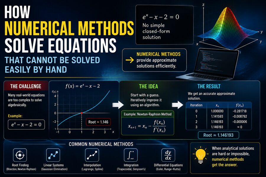
A faster technique is Newton’s method, also called the Newton–Raphson method.
Newton’s method uses the slope of the function to predict where the root is located.
The formula is:
xₙ₊₁ = xₙ − f(xₙ) / f′(xₙ)
where:
xₙ = current estimate
f(xₙ) = function value
f′(xₙ) = derivative
xₙ₊₁ = improved estimate
Suppose we again want to solve:
x² − 2 = 0
Then:
f(x) = x² − 2
and:
f′(x) = 2x
Choose an initial estimate:
x₀ = 1.5
Newton’s formula gives:
x₁ = 1.5 − (1.5² − 2)/(2 × 1.5)
which gives approximately:
x₁ = 1.41667
Perform another iteration:
x₂ ≈ 1.414216
Then:
x₃ ≈ 1.414214
In only a few calculations, the estimate becomes extremely accurate. ⚡
📐 The Geometry Behind Newton’s Method
Newton’s method has a beautiful geometric interpretation.
Start with a point on the function curve.
Draw the tangent line at that point.
The tangent line intersects the x-axis somewhere nearby.
Use that intersection as the next estimate.
Then repeat.
If the initial guess is good and the function behaves nicely, the estimates rapidly move toward the root.
This is why Newton’s method often converges much faster than bisection.
However, it is not guaranteed to work in every case.
A poor initial guess may cause the method to:
- Move away from the desired root
- Oscillate between values
- Reach a point where the derivative is zero
- Converge to a different root
So numerical algorithms involve trade-offs between speed, reliability, and computational cost.
🔄 Fixed-Point Iteration
Another important idea is fixed-point iteration.
Suppose an equation can be written as:
x = g(x)
We choose an initial guess and repeatedly calculate:
xₙ₊₁ = g(xₙ)
For example:
x = cos(x)
Choose:
x₀ = 1
Then:
x₁ = cos(1) ≈ 0.5403
x₂ = cos(0.5403) ≈ 0.8576
x₃ ≈ 0.6543
Continuing this process eventually produces values approaching:
0.739085…
This number is a fixed point because:
cos(0.739085…) ≈ 0.739085…
Not every fixed-point formulation converges, however. Engineers and mathematicians analyze the behavior of the function to determine whether repeated iteration will approach the solution.
🧩 Solving Systems of Many Equations
Numerical methods become even more important when many equations must be solved simultaneously.
Consider:
2x + y = 5
x − y = 1
This small system can be solved easily by hand.
But engineering models may contain thousands or even millions of equations.
For example, a simulation of airflow around an aircraft can divide the surrounding air into an enormous number of computational cells.
Each cell has variables such as:
- Pressure
- Velocity
- Temperature
- Density
These variables interact with neighboring cells, creating huge systems of equations.
Computers use numerical linear algebra techniques such as:
- Gaussian elimination
- LU decomposition
- Conjugate gradient methods
- Iterative matrix solvers
Without these techniques, modern scientific simulation would be practically impossible. ✈️💻
📈 Numerical Methods for Differential Equations
Many physical laws are expressed using differential equations.
Differential equations describe how quantities change.
For example, Newton’s law of motion can be written in differential form:
F = m(d²x/dt²)
Heat transfer, fluid flow, electrical circuits, population growth, chemical reactions, and planetary motion can all be described using differential equations.
Some differential equations have exact solutions.
Many do not.
Numerical methods approximate the solution at a sequence of points.
One simple method is Euler’s method.
Suppose:
dy/dx = f(x, y)
Euler’s method estimates the next value using:
yₙ₊₁ = yₙ + h f(xₙ, yₙ)
where h is a small step size.
The idea is to move forward using the current slope.
It is conceptually simple, but smaller step sizes are generally needed for better accuracy.
🏃 Runge–Kutta Methods
More sophisticated techniques improve upon Euler’s method.
One of the most famous is the fourth-order Runge–Kutta method, commonly called RK4.
Instead of estimating the slope only once during each step, RK4 evaluates the behavior of the function several times.
It then combines those slope estimates to obtain a much more accurate next value.
Runge–Kutta methods are widely used for problems involving:
- Vehicle dynamics 🚗
- Orbital mechanics 🛰️
- Chemical reactions ⚗️
- Control systems
- Electrical circuits
- Population models
- Mechanical systems
Numerical differential-equation solvers are among the foundations of modern engineering software.
🌊 Numerical Methods and Fluid Dynamics
Consider something as complicated as airflow around an airplane.
Air obeys mathematical equations known as the Navier–Stokes equations.
These equations describe how fluid velocity, pressure, density, and other variables change in space and time.
For realistic aircraft shapes, solving these equations exactly by hand is impossible.
Instead, engineers divide the region around the aircraft into many small cells or elements.
Computers then approximate the governing equations in each region.
This approach is known as Computational Fluid Dynamics, or CFD. 🌬️
CFD allows engineers to predict:
- Lift
- Drag
- Pressure distribution
- Turbulence
- Temperature
- Airflow separation
A modern aircraft can therefore undergo thousands of simulated aerodynamic tests before a physical prototype ever enters a wind tunnel.
🌉 Structural Engineering Also Depends on Numerical Approximation
Imagine predicting how a bridge bends under traffic and wind.
A real bridge contains complicated geometry, different materials, joints, supports, and varying loads.
It would be extremely difficult to represent the entire structure with one simple equation.
Engineers instead divide it into many smaller pieces called finite elements.
This technique is known as the Finite Element Method, or FEM.
Each element has relatively simple mathematical behavior.
The computer combines the equations from thousands or millions of elements to approximate the behavior of the full structure.
FEM is widely used to analyze:
- Bridges 🌉
- Buildings
- Aircraft
- Cars
- Turbines
- Medical implants
- Machine components
Numerical methods therefore allow engineers to solve problems that would otherwise be far too complicated for analytical mathematics.
🎯 Numerical Optimization
Sometimes the goal is not to solve one equation but to find the best possible solution.
Examples include:
- Minimizing fuel consumption
- Maximizing profit
- Reducing structural weight
- Improving aerodynamic efficiency
- Training machine-learning models
- Planning delivery routes
These are optimization problems.
A numerical algorithm searches through possible solutions and repeatedly attempts to improve the result.
One famous technique is gradient descent.
Gradient descent follows the direction in which a function decreases most rapidly.
Machine-learning systems frequently use gradient-based optimization to adjust millions or billions of parameters. 🤖
So even modern artificial intelligence depends heavily on numerical mathematics.
🧮 Why Computers Are Perfect for Numerical Methods
Many numerical algorithms involve a simple pattern:
- Start with an estimate.
- Perform calculations.
- Measure the error.
- Improve the estimate.
- Repeat until the error is small enough.
Humans can perform this process manually, but it becomes tedious after many iterations.
Computers are ideal for it because they can perform millions or billions of arithmetic operations rapidly.
A computer does not become bored calculating the same formula 100,000 times. 💻⚡
This ability transforms difficult mathematical problems into practical computational problems.
🎯 What Does “Convergence” Mean?
A numerical method converges when repeated calculations move closer to the true or desired solution.
For example:
1.4
1.41
1.414
1.4142
1.41421
These values are converging toward √2.
If the sequence instead behaves like:
1, 5, −20, 100, −700…
then the method is probably diverging.
Engineers must understand whether an algorithm is expected to converge before trusting its answer.
📏 When Should the Computer Stop Iterating?
A numerical algorithm could theoretically continue refining an answer indefinitely.
In practice, the computer uses a stopping criterion.
For example, it might stop when:
|xₙ₊₁ − xₙ| < 0.000001
This means the new answer differs from the previous one by less than one millionth.
Another method checks the residual:
|f(x)| < tolerance
If the equation requires:
f(x) = 0
then a very small value of f(x) indicates that the approximate solution is close to satisfying the equation.
The acceptable tolerance depends on the application.
A rough animation might tolerate relatively large errors.
A spacecraft navigation calculation may require much greater precision. 🛰️
⚠️ Numerical Errors Are Unavoidable
Numerical calculations are not perfectly exact.
Several types of error can occur.
✂️ Truncation Error
A numerical method may approximate an infinite mathematical process using a finite number of steps.
For example, Euler’s method approximates a curved solution using short straight-line steps.
The difference creates truncation error.
💻 Round-Off Error
Computers store numbers using finite numbers of bits.
Many decimal values cannot be represented exactly in binary floating-point form.
For example, the decimal number 0.1 typically cannot be represented perfectly in ordinary binary floating-point.
The computer stores a nearby approximation.
Usually this error is extremely small, but repeated calculations can sometimes amplify it.
🔬 Why Step Size Matters
Many numerical algorithms divide a problem into small steps.
Generally, smaller steps provide better approximations.
But smaller steps also require more computation.
Suppose a simulation covers 10 seconds.
Using:
1-second steps → 10 calculations
but:
0.001-second steps → 10,000 calculations
The second simulation may be more accurate, but it requires much more processing.
Numerical computing therefore involves balancing:
Accuracy ↔ computation time
Engineers aim to use enough resolution to obtain trustworthy answers without wasting excessive computational resources. ⚖️
🧠 Stability Is Just as Important as Accuracy
A numerical method can theoretically be accurate but behave badly under certain conditions.
Numerical stability describes how errors behave as calculations proceed.
A stable algorithm keeps small errors under control.
An unstable algorithm may amplify tiny rounding or approximation errors until the final result becomes meaningless.
This issue is especially important in:
- Weather models 🌦️
- Fluid simulations
- Structural dynamics
- Electrical simulations
- Long-duration calculations
Selecting a mathematically appropriate algorithm can therefore be just as important as using a powerful computer.
🌦️ Numerical Methods Predict the Weather
Weather forecasting is one of the largest everyday applications of numerical mathematics.
The atmosphere is governed by equations describing:
- Fluid motion
- Temperature
- Pressure
- Moisture
- Radiation
- Energy transfer
There is no practical closed-form solution for the entire atmosphere.
Meteorologists divide the atmosphere into a three-dimensional computational grid.
Supercomputers then numerically approximate how atmospheric conditions evolve over time.
The forecast on your phone is therefore ultimately the result of enormous systems of equations being solved approximately. 🌍☁️
🚀 Spacecraft Navigation Uses Numerical Computation
The movement of two isolated bodies under gravity can sometimes be described with elegant analytical equations.
But real spacecraft experience influences from:
- Multiple planets
- Moons
- Solar radiation pressure
- Atmospheric drag
- Irregular gravitational fields
- Engine burns
Numerical integration allows computers to predict a spacecraft’s trajectory under these complex conditions.
Mission planners can simulate where a spacecraft will be days, months, or years in the future.
Numerical methods have therefore helped guide probes across billions of kilometers of space. 🛰️🌌
🧪 Chemical Engineering Relies on Numerical Models
Chemical engineers use numerical methods to model:
- Chemical reactors
- Heat exchangers
- Distillation columns
- Fluid pipelines
- Reaction kinetics
- Process-control systems
For example, a chemical reactor may contain dozens of reactions occurring simultaneously.
The concentrations and temperatures may change every fraction of a second.
Numerical solvers allow engineers to predict the reactor’s behavior without solving the enormous coupled equation system by hand. ⚗️
🤖 Numerical Methods Behind Machine Learning
Machine learning also depends heavily on numerical methods.
Training a neural network means adjusting parameters so that the model’s prediction error becomes smaller.
There may be billions of parameters.
No human could solve such a system manually.
Instead, numerical optimization algorithms repeatedly:
make predictions → calculate error → adjust parameters → repeat
This process may occur trillions of times during the training of a large model.
Modern AI is therefore deeply connected to numerical mathematics. 🧠💻
🔍 How Do Engineers Know a Numerical Answer Is Correct?
A computer producing a number does not automatically mean that number is trustworthy.
Engineers verify numerical results in several ways.
They may:
- Compare with known analytical solutions
- Repeat the calculation using a finer grid
- Reduce the numerical step size
- Use a different algorithm
- Compare against experimental measurements
- Check conservation laws
- Estimate numerical error
For example, if a simulation gives nearly the same answer after doubling the grid resolution, confidence in the result increases.
This process is often called verification and validation.
Verification asks:
Did we solve the mathematical model correctly?
Validation asks:
Does the mathematical model accurately represent reality?
Both are essential.
🧠 Numerical Methods Do Not Replace Mathematics
It can be tempting to think that powerful computers eliminate the need for mathematical understanding.
The opposite is often true.
A computer will happily calculate the wrong equation millions of times.
Engineers still need mathematics to determine:
- Which equations describe the problem
- Which numerical method is appropriate
- Whether the algorithm will converge
- What error level is acceptable
- Whether the result is physically realistic
Numerical methods do not replace analytical reasoning.
They extend its reach. 🚀
🌟 Final Thoughts
Numerical methods allow mathematics to tackle problems that would otherwise be impossible or impractical to solve by hand.
Instead of demanding a perfect symbolic formula, numerical algorithms seek progressively better approximations.
Methods such as bisection, Newton’s method, iterative solvers, Runge–Kutta techniques, finite-element analysis, and numerical optimization turn difficult mathematical questions into sequences of manageable calculations. 🧮💻
This approach makes it possible to:
- Predict weather 🌦️
- Design aircraft ✈️
- Analyze bridges 🌉
- Simulate chemical plants ⚗️
- Navigate spacecraft 🛰️
- Model electrical systems ⚡
- Train artificial intelligence 🤖
The central idea is remarkably simple:
Start with an approximation, calculate how wrong it is, improve it, and repeat.
When repeated carefully with appropriate mathematics, this process can produce extraordinarily accurate answers to equations that have no convenient handwritten solution.
That is why numerical methods are among the most powerful bridges between pure mathematics and the real-world problems solved by modern computers. 🔢🌍