📐 How Partial Differential Equations Model Heat, Waves, and Fluid Flow

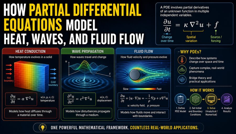
Many of the most important processes in physics do not depend on just one variable. Temperature changes from place to place and from one moment to the next. Waves move through space while changing over time. Fluids have velocity, pressure, and density that vary throughout a region. 🌡️🌊💨

To describe these changing systems mathematically, scientists and engineers use partial differential equations, usually abbreviated as PDEs.

A partial differential equation is an equation involving an unknown function of several variables and its partial derivatives. These derivatives describe how the function changes with respect to one variable while the others are held fixed.

For example, if temperature is written as:

T(x, y, z, t)

then temperature depends on three spatial coordinates and time.

A derivative such as:

∂T/∂t

describes how temperature changes with time at a particular location.

Meanwhile:

∂T/∂x

describes how temperature changes as we move in the x-direction at a particular instant.

By combining these derivatives with physical laws, PDEs can describe how heat spreads through metal, how sound travels through air, how water moves through pipes, how ocean waves propagate, and even how weather systems evolve. 🌍

🧠 What Makes a PDE Different From an Ordinary Differential Equation?

An ordinary differential equation, or ODE, usually involves a function of one independent variable.

For example, the position of a falling object might be represented as:

x(t)

where position depends only on time.

An ODE could describe how velocity changes with time.

A PDE, however, usually deals with quantities that depend on several variables.

For instance:

Temperature: T(x, y, z, t)
Pressure: p(x, y, z, t)
Fluid velocity: u(x, y, z, t)
Wave displacement: u(x, t)

This ability to describe changes over both space and time makes PDEs especially powerful for modeling continuous physical systems.

🌡️ The Heat Equation

One of the most famous partial differential equations is the heat equation.

In one spatial dimension, it can be written as:

∂T/∂t = α ∂²T/∂x²

where:

• T is temperature
• t is time
• x is position
• α is thermal diffusivity

Thermal diffusivity describes how quickly heat spreads through a material.

The equation says that the rate at which temperature changes over time depends on the curvature of the temperature distribution in space.

That may sound abstract, but the physical meaning is intuitive.

Heat tends to move from hotter regions toward colder regions. 🔥➡️❄️

If one part of a metal rod is much hotter than the surrounding region, heat flows outward from that region, causing the temperature differences to gradually smooth out.

🔥 A Simple Heat-Conduction Example

Imagine a long metal rod.

Initially, the left side is hot and the right side is cold.

At time:

t = 0

the temperature might change sharply along the rod.

As time passes, thermal energy spreads through the material.

The hot region cools while the cold region warms.

Eventually, if the rod is isolated from its surroundings, the temperature may approach a nearly uniform value.

The heat equation predicts how this smoothing happens.

Conceptually:

Sharp temperature differences ➡️ heat conduction ➡️ smoother temperature distribution

The stronger the temperature curvature in a region, the more rapidly the local temperature changes.

🧱 Why Material Properties Matter

Different materials conduct heat differently.

A metal such as copper spreads heat much more rapidly than a material such as wood or foam.

This behavior is reflected in parameters such as:

• Thermal conductivity
• Density
• Specific heat capacity
• Thermal diffusivity

In a more complete heat-transfer model, the equation may include internal heat generation or heat exchange with the environment.

For example, engineers can use heat-transfer PDEs to study:

🏠 Insulation in buildings
💻 Cooling of computer processors
🚗 Engine temperature
🔋 Battery thermal management
🔥 Industrial furnaces
🛰️ Spacecraft heat shields

The same fundamental mathematical ideas apply to all of them.

🌊 The Wave Equation

Another central PDE is the wave equation.

In one dimension, a common form is:

∂²u/∂t² = c² ∂²u/∂x²

where:

• u(x,t) represents displacement
• c is wave speed
• x is position
• t is time

This equation describes how disturbances propagate through space.

Unlike the heat equation, which tends to smooth out differences, the wave equation supports disturbances that travel.

Examples include:

• Vibrations on a string 🎸
• Sound waves 🔊
• Seismic waves 🌍
• Electromagnetic waves 📡
• Surface waves on water 🌊

🎸 A Vibrating String

Consider a guitar string fixed at both ends.

If the string is pulled upward and released, it vibrates.

The displacement of the string depends on both position and time:

u(x,t)

At each instant, different points on the string may have different vertical positions.

The wave equation predicts how these displacements evolve.

The disturbance travels along the string, reflects from the fixed ends, and interferes with itself.

Certain vibration patterns become especially important.

These are known as normal modes or standing waves.

The frequencies of these modes depend on:

• String length
• Tension
• Mass per unit length

This is why changing the tension of a guitar string changes its musical pitch. 🎵

🔊 Sound as a PDE Problem

Sound also involves waves.

When a speaker vibrates, it compresses and expands nearby air.

These pressure disturbances propagate outward.

The pressure field might be written as:

p(x, y, z, t)

A wave equation can then describe how acoustic pressure changes through space and time.

Engineers use acoustic PDEs to design:

🎧 Headphones
🎤 Microphones
🏟️ Concert halls
🚗 Vehicle interiors
✈️ Aircraft cabins
🔊 Loudspeakers

They can simulate how sound reflects from walls, passes through openings, and interferes with other waves.

🌊 Boundary Conditions Matter

A PDE by itself is usually not enough to determine a unique solution.

Scientists also need boundary conditions and often initial conditions.

Initial conditions describe the state of the system at the starting time.

For example:

T(x,0) = initial temperature distribution

Boundary conditions describe what happens at the edges of the region.

For a heat problem, a boundary might be:

T(0,t) = 100°C

meaning one end of a rod is held at 100°C.

For a vibrating string, fixed ends might require:

u(0,t) = 0
u(L,t) = 0

meaning the ends cannot move.

Boundary conditions are essential because the same PDE can produce very different solutions depending on how the system is constrained. 📏

💨 Fluid Flow and PDEs

Fluid dynamics is one of the most important and challenging applications of partial differential equations.

A fluid such as air or water has properties that vary continuously through space.

These can include:

• Velocity
• Pressure
• Density
• Temperature
• Viscosity

The velocity field may be written as:

u(x, y, z, t)

This means that every point in the fluid can have its own velocity at every moment.

To predict the motion of the fluid, engineers use equations based on conservation laws.

⚖️ Conservation of Mass

One fundamental principle is conservation of mass.

Mass cannot simply disappear.

For an incompressible fluid, a common mathematical condition is:

∇ · u = 0

This equation says that the velocity field has zero divergence.

Physically, it means that for a small fluid region, the amount of fluid flowing in must balance the amount flowing out.

For compressible fluids, such as high-speed gases, a more general equation called the continuity equation accounts for changes in density.

🌪️ The Navier-Stokes Equations

The most famous equations of fluid mechanics are the Navier-Stokes equations.

A simplified form for an incompressible Newtonian fluid is:

ρ(∂u/∂t + u · ∇u) = -∇p + μ∇²u + f

where:

• ρ is density
• u is velocity
• p is pressure
• μ is dynamic viscosity
• f represents body forces such as gravity

This compact equation describes several competing effects.

The term:

∂u/∂t

represents how velocity changes with time.

The nonlinear term:

u · ∇u

describes how fluid motion carries momentum from one place to another.

The pressure term:

-∇p

describes acceleration caused by pressure differences.

The viscosity term:

μ∇²u

describes internal friction that smooths velocity differences.

Together, these terms describe the complex behavior of real fluids. 💨

✈️ Why Fluid PDEs Matter in Engineering

Navier-Stokes equations are used throughout engineering.

They help model:

✈️ Airflow around aircraft wings
🚗 Aerodynamics around vehicles
🚀 Rocket exhaust
🌊 Ocean currents
🌬️ Atmospheric circulation
🩸 Blood flow
🏭 Chemical reactors
🚰 Water pipelines
🌀 Turbulence

Aircraft designers, for example, need to understand how air pressure and velocity change around a wing.

Those pressure differences generate lift and drag.

By solving fluid-flow PDEs numerically, engineers can test designs virtually before constructing physical prototypes.

🌀 Why Turbulence Is So Difficult

Fluid flow becomes especially difficult when it is turbulent.

Turbulence contains swirling structures over many different size scales.

Large eddies break into smaller eddies, which break into even smaller structures.

The flow can change rapidly and unpredictably.

The Navier-Stokes equations still describe the fluid, but solving them accurately can require enormous computational resources.

This is why computational fluid dynamics, or CFD, is such an important field.

Rather than solving the equations with simple formulas, computers approximate the solution at millions or even billions of points.

💻 Numerical Solutions to PDEs

Only a limited number of PDEs have simple exact solutions.

Real engineering geometries are often too complicated.

A turbine blade, weather system, blood vessel, or aircraft fuselage does not have the simple shape needed for an easy analytic solution.

Instead, scientists use numerical methods.

The physical region is divided into many small pieces.

The PDE is then approximated by algebraic equations that computers can solve.

Common numerical approaches include:

• Finite difference method
• Finite element method
• Finite volume method
• Spectral methods

Each method represents the continuous PDE problem in a form suitable for computation. 🖥️

🔢 Finite Difference Method

The finite difference method approximates derivatives using values at nearby grid points.

For example, instead of calculating an exact derivative, the computer may approximate:

∂T/∂x ≈ [T(x+Δx) – T(x)] / Δx

The spatial region is divided into a grid.

The computer repeatedly updates temperatures, velocities, or other quantities at those grid points.

This approach is conceptually straightforward and is often used in structured geometries.

🔺 Finite Element Method

The finite element method, or FEM, divides a complicated region into smaller elements such as triangles or tetrahedra.

Instead of solving the PDE globally in one step, the method approximates the solution within each element.

The results are then connected across the entire geometry.

Finite element methods are especially popular for:

🏗️ Structural mechanics
🌡️ Heat transfer
⚡ Electromagnetics
💧 Fluid flow
🧱 Materials engineering

They are powerful because they can handle irregular shapes and complex boundary conditions.

📦 Finite Volume Method

The finite volume method is widely used in fluid dynamics.

It divides the flow region into many small control volumes.

Conservation laws are applied to each one.

For each cell:

Amount entering – amount leaving = change inside

This makes finite volume methods particularly well suited to conserving mass, momentum, and energy.

Many CFD programs use this approach.

🧮 PDE Classification

Many second-order PDEs can be classified into three broad categories:

Elliptic
Parabolic
Hyperbolic

These categories are associated with different physical behaviors.

🌡️ Parabolic Equations

The heat equation is a classic parabolic PDE.

Parabolic equations often describe diffusion-like processes where disturbances smooth out over time.

Examples include heat conduction and certain forms of material diffusion.

🌊 Hyperbolic Equations

The wave equation is hyperbolic.

Hyperbolic PDEs describe disturbances that propagate at finite speeds.

Examples include sound waves, elastic waves, and many equations used in compressible flow.

⚡ Elliptic Equations

Laplace’s equation:

∇²u = 0

is elliptic.

Elliptic equations often describe equilibrium or steady-state distributions.

They appear in electrostatics, steady heat conduction, gravitational potentials, and incompressible flow problems.

Understanding the classification helps mathematicians choose appropriate solution methods.

🧊 Diffusion Versus Waves

The difference between heat and wave behavior is mathematically striking.

Suppose we create a sharp disturbance.

In heat diffusion:

Disturbance ➡️ spreads and smooths out

In a wave:

Disturbance ➡️ travels through the medium

For heat, information effectively diffuses outward.

For waves, the disturbance maintains a propagating structure.

The form of the PDE determines which physical behavior emerges.

This illustrates one of the most remarkable features of mathematics: a relatively compact equation can encode an entire class of physical behavior. 📐✨

🌍 Coupled PDEs Model Complex Systems

Real systems often involve several physical processes simultaneously.

A jet engine, for example, can involve:

• Fluid flow
• Heat transfer
• Combustion
• Chemical reactions
• Turbulence
• Structural heating

These processes influence one another.

Temperature affects density.

Density affects fluid flow.

Fluid motion transports heat.

Chemical reactions release energy.

Engineers therefore solve coupled PDE systems in which several equations interact.

The mathematics becomes more difficult, but the models can capture remarkably detailed physical behavior.

🌦️ PDEs in Weather Prediction

Weather forecasting is another enormous PDE problem.

The atmosphere is a moving fluid affected by:

🌡️ Temperature
💨 Wind
💧 Moisture
🌍 Earth’s rotation
☀️ Solar heating
☁️ Phase changes of water

Weather models divide the atmosphere into a three-dimensional computational grid.

PDEs describing fluid motion, thermodynamics, moisture transport, and radiation are solved repeatedly.

The result is a prediction of how atmospheric conditions will evolve.

Modern weather forecasting would be impossible without numerical PDE methods and high-performance computing.

🩺 PDEs in Medicine

Partial differential equations are also used in biology and medicine.

Examples include modeling:

🩸 Blood flow through arteries
💊 Drug diffusion through tissue
🧠 Electrical activity in the heart and brain
🫁 Airflow through lungs
🌡️ Heat treatment of tumors

A blood-flow model, for instance, may use fluid-dynamics PDEs combined with equations describing flexible blood-vessel walls.

Such models can help researchers study cardiovascular conditions or evaluate medical-device designs.

⚡ PDEs Beyond Heat, Waves, and Fluids

The reach of PDEs extends far beyond the three classic examples.

They appear in:

⚡ Maxwell’s equations for electromagnetism
⚛️ Schrödinger’s equation in quantum mechanics
💹 Mathematical finance
🧬 Reaction-diffusion systems
🌌 General relativity
🧱 Elasticity and solid mechanics
🌊 Groundwater flow
🔥 Combustion
🛰️ Plasma physics

Whenever a physical quantity varies through both space and time, a PDE is often nearby.

🎯 Models Are Approximations of Reality

A mathematical model is not the physical world itself.

Engineers must decide which effects are important enough to include.

For example, a simple heat equation may assume:

• Constant material properties
• No internal heat source
• Uniform geometry
• No phase changes

A more sophisticated model can remove some of those assumptions.

The challenge is balancing realism and computational cost.

A model that includes every microscopic detail may be impossible to compute.

A model that is too simple may miss important behavior.

Good modeling therefore involves choosing equations and approximations appropriate for the problem. ⚖️

🧪 Experiments Remain Essential

Even highly sophisticated PDE simulations need experimental validation.

Engineers compare predictions with real measurements.

For example, a CFD model of an aircraft wing may be compared with data from a wind tunnel.

A heat-transfer simulation may be checked using temperature sensors.

If the results disagree, researchers may adjust:

• Material properties
• Boundary conditions
• Numerical resolution
• Turbulence models
• Physical assumptions

Mathematics, computation, and experiment therefore work together.

🚀 Why PDEs Are So Powerful

Partial differential equations are powerful because they translate local physical laws into global predictions.

A PDE may describe what happens at one infinitesimal point:

How does temperature change here?

How does pressure accelerate fluid here?

How does the string curvature affect acceleration here?

When these local rules are applied everywhere, they predict the behavior of the entire system.

That is why PDEs can describe phenomena ranging from a tiny vibrating membrane to the atmosphere of an entire planet. 🌍

🏁 Conclusion

Partial differential equations are among the most important mathematical tools in science and engineering because they describe quantities that vary across both space and time.

The heat equation models diffusion by explaining how temperature differences gradually smooth out. 🌡️

The wave equation describes disturbances that propagate through space, such as sound, vibrations, and electromagnetic waves. 🌊

The Navier-Stokes equations model fluid motion by combining conservation of momentum with pressure, viscosity, and fluid acceleration. 💨

These equations can be simple to write but extremely difficult to solve.

For idealized cases, mathematicians can sometimes find exact formulas. For realistic systems, engineers typically use numerical methods such as finite differences, finite elements, and finite volumes.

Powerful computers then approximate the solutions across enormous grids containing millions of interacting points.

Whenever engineers predict the temperature of a turbine blade, simulate airflow around an aircraft, model ocean currents, design a concert hall, forecast the weather, or analyze blood flow, partial differential equations are helping transform physical laws into quantitative predictions. 🧠💻

In essence:

Physical law + spatial change + time evolution = partial differential equation

And by solving those equations, scientists can understand, predict, and design some of the most complex systems in the natural and engineered world. 📐🌍✨