
An engineer runs a structural model and finds that changing a load value in the sixth decimal place changes a predicted displacement by several percent. The software has not necessarily failed. The model may be warning that the calculation is highly sensitive to its inputs.
In another setting, a sensor-calibration routine produces coefficients that look implausibly large. A design optimisation changes direction between iterations, even though the objective function appears smooth. A least-squares fit matches the measured data but makes poor predictions for new operating conditions.
These situations can share one underlying mathematical feature: the problem is ill-conditioned. Small uncertainty, rounding, measurement noise, or modelling variation can be amplified into a large change in the computed answer.
The condition number gives engineers a practical way to measure that sensitivity. It does not say whether a model is physically correct, but it can reveal whether apparently precise numerical results deserve trust.
🧭 1. The central idea of conditioning
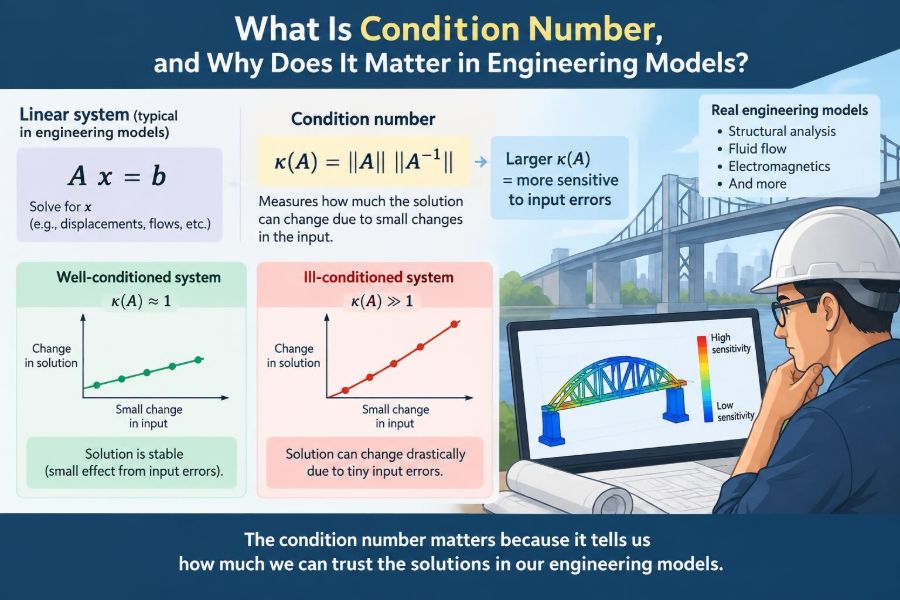
Conditioning describes a property of a mathematical problem: how much its answer changes when its input changes slightly. A well-conditioned problem changes proportionally; an ill-conditioned problem can react dramatically.
The condition number is a numerical measure of this sensitivity. In broad terms, a value near 1 is reassuring, while a much larger value signals potential amplification of input errors.
Conditioning belongs to the problem itself, not merely to the computer program used to solve it. That distinction is essential in engineering analysis. 🔍
📏 2. A simple relative-error definition
Suppose a problem maps input x to output y = f(x). For small perturbations, the relative condition number asks how large the relative output change can be compared with the relative input change.
relative condition number ≈ (relative change in output) / (relative change in input)
If a 0.01% input uncertainty can produce roughly a 1% output uncertainty, the local condition number is about 100. The calculation has amplified the relative uncertainty by two orders of magnitude.
This is usually a local statement, valid near a particular operating point. Nonlinear engineering models can have very different conditioning in different regions.
🧮 3. Condition number for a linear system
Many engineering computations reduce to solving Ax = b, where A is a matrix, b is the known load, source, or measurement vector, and x is the unknown response.
For an invertible matrix, a common matrix condition number is:
κ(A) = ||A|| · ||A⁻¹||
The symbol κ, pronounced “kappa,” denotes the condition number. The selected matrix norm matters, so a condition number should ideally be reported with its norm, such as the 2-norm or infinity norm.
In the 2-norm, κ₂(A) has a particularly useful interpretation through singular values.
🔢 4. Why a condition number cannot be below one
For any invertible matrix and any consistent induced norm, κ(A) ≥ 1. A condition number of 1 represents the best possible scaling of directional sensitivity in that norm.
It does not mean every engineering uncertainty disappears. Measurements may still be noisy, material properties may be uncertain, and the governing equations may be incomplete.
It means the matrix operation itself does not preferentially magnify some input directions more than others. That is a valuable but limited assurance.
📐 5. Singular values provide the clearest picture
For the 2-norm, the condition number is the ratio of the largest to the smallest singular value:
κ₂(A) = σmax(A) / σmin(A)
Singular values describe how a matrix stretches or compresses vectors in different directions. A large largest singular value means one direction is strongly amplified; a tiny smallest singular value means another direction is nearly collapsed.
When σmin is close to zero, small disturbances in the corresponding output direction require very large changes in the solution. This is the geometric heart of ill-conditioning.
🗺️ 6. The geometry behind the formula
Imagine applying a matrix to a unit circle. A well-conditioned transformation turns it into a shape that is still fairly round. An ill-conditioned transformation turns it into a long, thin ellipse.
Along the thin direction, different input vectors become difficult to distinguish after transformation. Reversing the transformation then becomes sensitive: a tiny movement in the transformed space can imply a substantial movement in the original space.
This explains why inversion, parameter estimation, and reconstruction problems are often vulnerable. They attempt to recover information from directions that the model has nearly erased.
🏗️ 7. A structural-analysis example
In a finite-element structural model, the equilibrium equation is often written K u = f. Here K is the stiffness matrix, u contains nodal displacements, and f contains applied forces.
A nearly singular stiffness matrix may arise when a structure has an unconstrained rigid-body motion, an unintended mechanism, or an extreme contrast between stiffness values. In that case, small load or modelling changes can produce large displacement changes.
The condition number helps distinguish a robustly restrained system from one that is mathematically close to a free motion. It should prompt engineering inspection, not automatic acceptance.
🌡️ 8. Heat transfer and diffusion models
Steady heat-conduction models also produce linear systems. Their conditioning is influenced by mesh resolution, boundary conditions, geometry, and contrasts in thermal conductivity.
A very fine mesh can increase the spread of relevant matrix scales, while highly heterogeneous materials can create numerically difficult directions. Similar effects occur in groundwater flow, electrostatics, and diffusion-reaction models.
Ill-conditioning does not prove that a refined mesh is wrong. It means that discretisation choices, solver settings, and result verification deserve extra care.
📡 9. Why inverse problems are especially sensitive
Forward models predict observations from known parameters. Inverse problems work backward: they infer material properties, source locations, loads, or states from measured responses.
The backward step is often ill-conditioned because different parameter combinations can produce very similar observations. Sensor noise then makes it difficult to identify which combination is physically correct.
- Estimating a heat source from temperature measurements
- Identifying stiffness parameters from vibration data
- Reconstructing an image or field from indirect measurements
- Calibrating constitutive-model parameters from experiments
A large condition number reveals weak identifiability in the chosen data and parameterisation.
📊 10. Least squares and the design matrix
In linear regression, engineers often solve min ||Ax - b||₂. The columns of A represent predictors, basis functions, or sensitivity directions.
If two columns are nearly dependent, the data cannot clearly separate their corresponding coefficients. The fit may remain good while individual estimated coefficients become unstable.
This issue is called multicollinearity in statistical modelling. In engineering terms, it can mean that a test campaign did not excite independent physical effects strongly enough.
🧪 11. Nearly dependent columns in practice
Suppose a model uses two predictors that vary together over all experiments. Their individual effects may be impossible to estimate reliably, even if their combined effect is well determined.
For example, a test plan might change temperature and pressure together every time. A fitted model can struggle to separate temperature sensitivity from pressure sensitivity because the observations contain little independent evidence.
The remedy is often experimental design, not a more elaborate solver. Add informative operating points, broaden ranges safely, or measure additional response variables.
⚖️ 12. Conditioning is not the same as accuracy
A condition number measures sensitivity to perturbations. It does not directly measure the total error in an engineering answer.
A well-conditioned model may still be inaccurate because its geometry, loading, material law, boundary conditions, or assumptions are wrong. Conversely, an ill-conditioned problem may yield a useful answer if inputs are very accurate and uncertainty is carefully managed.
Think of conditioning as a risk multiplier. It indicates how readily unavoidable imperfections can become consequential.
🖥️ 13. Conditioning is not the same as solver stability
Numerical stability describes an algorithm. A stable algorithm controls the extra errors introduced during computation; an unstable one can create large errors even for a well-conditioned problem.
Conditioning describes the problem. Even the best stable algorithm cannot guarantee many correct digits when the underlying problem is severely ill-conditioned.
| Question | Conditioning | Numerical stability |
|---|---|---|
| Property of | The mathematical problem | The algorithm or implementation |
| Main concern | Input-error amplification | Computational-error amplification |
| Typical response | Reformulate, redesign, regularise | Use a better numerical method |
Reliable engineering computation requires attention to both.
🧾 14. Forward error and backward error
Forward error compares the computed answer with the exact answer to the original problem. It is what users usually care about, but the exact answer is often unavailable.
Backward error asks a different question: for what small perturbation of the input would the computed answer be exact? A small backward error means the algorithm solved a nearby problem accurately.
For an ill-conditioned problem, a tiny backward error can still correspond to a substantial forward error. The approximate relationship is that forward error may scale with condition number times backward error.
🧩 15. Residuals can be misleading
For Ax = b, the residual is r = b - A x̂, where x̂ is the computed solution. A small residual is useful evidence that the equations are nearly satisfied.
But a small residual does not always mean that x̂ is close to the true solution. If A is ill-conditioned, distinctly different solution vectors can produce nearly the same right-hand side.
Check residuals, but also inspect conditioning, physical plausibility, constraints, and sensitivity to realistic input variations.
🔍 16. Interpreting the size of κ
There is no universal threshold at which a condition number becomes unacceptable. The impact depends on input uncertainty, arithmetic precision, the required output accuracy, and the consequences of a wrong decision.
A condition number of 100 may be harmless for a screening calculation and concerning for a tightly controlled calibration. A value of one million may be manageable with high-quality data and careful regularisation, or fatal when inputs are noisy.
Use orders of magnitude as a prompt for investigation rather than treating any single cutoff as a law.
💻 17. Digits, floating-point arithmetic, and lost precision
Finite-precision arithmetic stores only a limited number of significant digits. If a problem has condition number roughly 10ᵏ, it can potentially consume about k digits of relative accuracy in an unfavorable case.
This is a rule of thumb, not a guaranteed digit count. Algorithm choice, scaling, input errors, and the specific right-hand side all influence the observed result.
Higher precision can reduce roundoff error, but it cannot fix uncertain measurements or a fundamentally non-identifiable model.
📦 18. Units and scaling can change the numerical picture
Engineering variables commonly have very different magnitudes: lengths in millimetres, forces in kilonewtons, temperatures in degrees, and stiffnesses in much larger numerical units. Poorly scaled equations can create avoidable numerical difficulty.
Rescaling variables and equations so typical quantities are closer in magnitude can improve solver behavior and make diagnostics more meaningful. Nondimensionalisation often achieves the same goal while highlighting governing physical ratios.
However, scaling must be interpreted carefully. It can improve a matrix condition number without resolving genuine physical non-identifiability.
🔧 19. Row scaling and column scaling
Row scaling balances equations; column scaling balances unknowns. Both can reduce numerical disparities that arise solely from units or arbitrary parameter magnitudes.
In parameter estimation, scaling columns by meaningful parameter ranges makes it easier to compare sensitivities. A parameter with a small numerical unit should not appear unimportant merely because of its chosen representation.
Always document the scaling used when reporting conditioning. Otherwise, colleagues may compare values that describe different coordinate systems.
🧱 20. Mesh refinement can affect conditioning
As a finite-element mesh is refined, the discrete system often contains modes over a wider range of spatial scales. This can increase conditioning difficulty, particularly for elliptic problems such as diffusion and linear elasticity.
That does not mean engineers should avoid convergence studies. Mesh refinement is necessary to control discretisation error, but it may require better preconditioners and more robust iterative methods.
The key lesson is that accuracy goals interact: a finer model can reduce one error source while making another more visible.
🚧 21. Boundary conditions deserve immediate attention
Unexpectedly large condition numbers in mechanics often point toward boundary-condition problems. Missing constraints can leave rigid-body modes, while redundant or incompatible constraints can also distort the formulation.
In thermal, electrical, and fluid models, disconnected regions or insufficient reference conditions can create related difficulties. A singular matrix is the extreme case: the solution is not unique or may not exist under the stated equations.
Before tuning a solver, check the physical connectivity and the mathematical completeness of constraints.
🧠 22. Preconditioning changes the solve, not the physics
For large sparse systems, iterative solvers often use a preconditioner: a matrix or operation that makes the transformed system easier to solve. Good preconditioning can greatly accelerate convergence.
Conceptually, it changes the numerical landscape seen by the algorithm. It does not change the intended physical solution when applied correctly.
Preconditioning should not be confused with curing an ill-posed inference problem. It can improve computational efficiency while parameter uncertainty remains large.
🛡️ 23. Regularisation manages unstable estimation
When data cannot uniquely determine a solution, regularisation adds justified preference for smoother, smaller, or physically plausible solutions. A common form is:
min ||Ax - b||₂² + λ||Lx||₂²
The parameter λ controls the trade-off between fitting the data and enforcing the added preference. Regularisation can stabilize inverse problems, but it introduces bias and must be chosen transparently.
Physical constraints, prior knowledge, and validation data are often more defensible than arbitrary numerical smoothing.
🧭 24. Better data can beat more computation
If ill-conditioning comes from weakly informative measurements, collecting more of the same type of data may provide limited benefit. What matters is whether new data distinguish the uncertain directions in parameter space.
Useful design questions
- Which parameters produce nearly indistinguishable responses?
- Which operating conditions separate those responses?
- Can sensor locations be changed to observe missing modes?
- Can a controlled input excite the system more independently?
Condition-number analysis can therefore guide test design as well as numerical implementation.
📈 25. Practical diagnostics for engineering workflows
Do not rely on one diagnostic alone. Combine numerical checks with model review and domain knowledge.
- Estimate a suitable condition number for important matrices or Jacobians.
- Inspect singular values, not just their ratio, when possible.
- Monitor residuals and solver convergence separately.
- Perturb loads, measurements, and material inputs within credible ranges.
- Compare solutions across mesh levels, scalings, and formulations.
- Check whether estimated parameters remain physically plausible.
A sensitivity study often turns an abstract warning into a clear engineering decision.
🧰 26. Computing a condition number sensibly
Most numerical environments provide routines to estimate matrix condition numbers. For small dense matrices, a singular-value decomposition gives a direct and informative 2-norm calculation.
For large sparse matrices, explicitly forming an inverse is usually unnecessary and often undesirable. Estimation routines, iterative methods, and problem-specific spectral analysis are typically more practical.
Report what was computed: matrix definition, norm, scaling, approximation method, and operating point. A bare condition number without context can be easy to misread.
✅ 27. The core principle: sensitivity sets the confidence limit
The condition number answers a disciplined question: if the inputs are slightly wrong, how much can the answer move? It connects numerical linear algebra to measurement quality, model formulation, experiment design, and engineering judgement.
A high condition number is not a verdict that a model must be discarded. It is a signal to examine constraints, scales, data independence, discretisation, algorithms, and the uncertainty attached to reported results.
The most useful engineering result is not merely a computed number, but a number accompanied by an honest understanding of how sensitive it is. 📐🔎🛠️