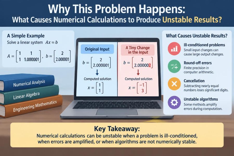

A simulation of a bridge begins to vibrate wildly even though the physical model should settle down. A spreadsheet changes from a sensible answer to an absurd one after a few copied formulas. A machine-learning routine works for one data set, then returns NaN for another.
These failures often look like programming bugs. Sometimes they are. But many arise from a more fundamental issue: computers calculate with finite precision, while mathematical formulas are usually written as though every number were exact.
That gap matters whenever calculations are repeated, data span very different scales, or a model contains nearly cancelling quantities. A result can be numerically unstable even when the underlying equation is correct and the code follows it exactly.
Understanding why instability happens makes numerical work easier to diagnose. It also helps engineers choose algorithms, scales, tolerances, and checks that produce answers they can trust.
🧭 What “unstable” means in numerical work
A numerical calculation is unstable when small unavoidable changes in its inputs or intermediate arithmetic produce disproportionately large changes in its output. Those small changes may come from rounding, measured-data uncertainty, or tiny differences in the order of operations.
There are two related ideas. Problem conditioning asks whether the mathematical problem itself is sensitive. Algorithmic stability asks whether a particular computational method amplifies errors unnecessarily. A stable algorithm cannot fully rescue a severely sensitive problem, but an unstable algorithm can ruin an otherwise manageable one.
🖥️ Computers do not store most real numbers exactly
Most engineering software uses floating-point numbers. They represent values with a sign, a limited number of significant binary digits, and an exponent. This efficiently covers huge ranges, but it cannot represent every real number—or even every familiar decimal—exactly.
For example, a decimal such as 0.1 generally has no finite binary representation. The stored value is a nearby approximation. One approximation is usually harmless; millions of arithmetic operations on approximations may not be.
🔢 Rounding is built into every finite-precision operation
After an addition, multiplication, division, or function evaluation, the exact mathematical result may not fit in the available floating-point format. It is rounded to the nearest representable value. The difference is called roundoff error.
Roundoff is not evidence that a computer is malfunctioning. It is the normal price of finite storage. Numerical analysis asks whether an algorithm lets these tiny local errors remain small or repeatedly magnifies them.
📏 Absolute error and relative error tell different stories
Absolute error is the difference between an approximation and a reference value. Relative error divides that difference by the size of the reference value, when the reference is nonzero.
An error of 0.001 is negligible for a length near 1000 m, but serious for a thickness near 0.0001 m. Relative error is often more informative for engineering quantities because it reflects the scale of the result. Near zero, however, relative error can become misleadingly large, so absolute tolerances are also needed.
💥 Catastrophic cancellation destroys useful digits
Cancellation occurs when subtracting nearly equal numbers. The leading digits match and disappear, leaving a small difference whose remaining digits may contain mostly prior rounding error.
Suppose two computed quantities are both about 1,000,000 but differ by 0.01. If each quantity is only reliable to a few decimal places, their subtraction may provide a poor estimate of 0.01. The issue is not that subtraction is forbidden; it is that the desired answer is much smaller than the quantities being subtracted.
🧮 A familiar formula can be a poor calculation
The quadratic formula illustrates this distinction. For ax² + bx + c = 0, directly evaluating (-b + √(b² - 4ac))/(2a) can suffer severe cancellation when b is positive and the square root is close to b.
A better approach computes the root without cancellation first, then obtains the other from the relation x₁x₂ = c/a. Algebraically equivalent formulas do not necessarily have equivalent numerical behavior. Choosing the right form is often the first repair.
📈 Error accumulation grows in long computations
A calculation with many steps has many opportunities for rounding error. Summing sensor readings, stepping a differential equation forward, or multiplying long chains of matrices can all accumulate small discrepancies.
Accumulation is not always linear. If later operations feed on earlier approximations, errors may interact and grow faster. Repeated addition of a tiny value to a very large running total can even stop changing the total once the tiny increment falls below the spacing between representable numbers at that magnitude.
🔁 Feedback loops can amplify numerical noise
Recurrences are especially vulnerable because each new value depends on previous computed values. In a stable recurrence, small perturbations decay or remain bounded. In an unstable recurrence, they grow with every iteration.
This matters in time-stepping models, digital filters, control simulations, and iterative matrix methods. A physically damped system can appear to gain energy if the numerical update rule has the wrong stability properties for the chosen time step.
⏱️ Time steps that are too large miss the dynamics
Differential equations describe continuous change, but a computer samples that change in discrete increments. Explicit methods are often convenient, yet they can become unstable when the time step is too large relative to the fastest process in the model.
For a stiff thermal, chemical, or mechanical model, slow behavior may coexist with very fast decay. A step size that looks reasonable for the slow motion can destabilize the fast mode. Reducing the step can help, but a method designed for stiff systems may be more efficient.
🧱 Stiffness is a scale-separation problem
A system is commonly called stiff when it contains components evolving on very different time scales. The solution may change slowly overall while still containing rapidly decaying modes that restrict simple numerical methods.
The practical symptom is frustrating: an explicit solver requires extremely small steps for stability, even when the plotted solution looks smooth. Implicit methods require more work per step, but they can often take much larger stable steps. The appropriate choice depends on accuracy needs and model structure.
🗂️ Ill-conditioned matrices make solutions sensitive
In a linear system Ax = b, the matrix A determines how errors in b affect x. If columns of A are nearly dependent, many combinations of unknowns explain the data almost equally well. Then small perturbations can cause large changes in the computed parameters.
The condition number summarizes this sensitivity for a chosen norm. A large condition number is a warning, not a complete diagnosis: it indicates that input uncertainty and roundoff may be amplified, particularly when the requested answer needs many reliable digits.
📐 Nearly parallel directions cause geometric ambiguity
Ill-conditioning has a useful geometric interpretation. Imagine estimating the intersection of two nearly parallel lines. A tiny change in either slope can move their intersection a long distance.
Regression with highly correlated predictors has the same flavor. The model may predict outputs reasonably well, while the individual fitted coefficients vary dramatically. The instability belongs partly to the information in the data, not merely to the solver.
🧪 Noisy measurements enter before the algorithm begins
Numerical precision cannot create information that measurements do not contain. Instrument noise, calibration drift, digitization, and uncertain boundary conditions all perturb model inputs before computation starts.
When a problem is sensitive, reporting many output digits can give a false impression of certainty. Compare output changes against plausible input variation, not just against a software tolerance. A tightly converged iteration may still be converging to an answer that is physically uncertain.
📊 Poor scaling makes arithmetic work harder
Variables with vastly different magnitudes can make systems difficult to solve. For instance, a model may combine a displacement in micrometres, a force in kilonewtons, and a modulus in gigapascals. The physics can be valid while the numerical representation is awkward.
Scaling rewrites variables or equations so typical values are closer to one another, often near unity. Nondimensionalization goes further by expressing a model through meaningful reference scales. This can improve conditioning, make tolerances interpretable, and reveal which effects actually dominate.
⚖️ Units can hide numerical trouble
Changing units does not change the physical answer, but it can change intermediate magnitudes substantially. A formula evaluated in metres may behave differently in floating-point arithmetic from the same formula evaluated in millimetres, especially if it contains subtraction or powers.
Use a consistent unit system, and inspect the order of magnitude of every variable. Unit consistency prevents physical mistakes; good scaling reduces numerical sensitivity. They overlap, but they are not the same task.
🧩 Subtractive formulas often have better alternatives
When cancellation is likely, look for identities or specialized functions that preserve accuracy. For small x, evaluating exp(x) - 1 directly can lose significant digits; many numerical libraries provide expm1(x) for this case. Likewise, log1p(x) is designed for log(1+x) when x is small.
Rationalizing expressions, factoring common terms, or using series expansions in a justified small-parameter regime can also help. The goal is not symbolic elegance. It is to avoid forming a tiny answer by subtracting two poorly known large ones.
➕ Summation order changes the answer
Real-number addition is associative, but floating-point addition is not: (a+b)+c can differ from a+(b+c). This becomes visible when values have mixed magnitudes or signs.
Summing from smaller magnitudes to larger ones often retains more small contributions. Pairwise summation and compensated methods, such as Kahan-style summation, track lost low-order information more carefully. Parallel programs should be expected to show small run-to-run differences when reductions occur in different orders.
🧮 Direct solvers need numerically safe factorizations
Solving equations by explicitly forming an inverse is usually less accurate and less efficient than solving the system through a factorization. For general dense systems, pivoted LU factorization is common; for least squares, QR factorization is often safer than forming normal equations.
Normal equations square the condition number in a typical sense, so they can worsen sensitivity. Singular value decomposition is more expensive but particularly informative when rank deficiency or near-dependence is suspected. Solver choice should follow matrix structure, not habit.
🔄 Iterative methods can converge, stall, or diverge
Iterative solvers refine an estimate repeatedly. Their behavior depends on the spectrum and structure of the system, the initial guess, stopping rule, and often a preconditioner—a transformation that makes the system easier for the iteration.
A small residual does not always mean a small solution error, especially for ill-conditioned matrices. Conversely, slow residual reduction may reflect a poor formulation rather than an incorrect physical model. Monitor both the residual and quantities that matter to the engineering decision.
🎯 Tolerances are engineering choices, not magic numbers
An absolute tolerance alone can be too strict for large quantities and too loose near zero. A relative tolerance alone becomes troublesome when the target is close to zero. Robust stopping tests commonly combine both.
Choose tolerances from required output accuracy, input uncertainty, scale, and cost—not from the number of digits displayed by software. Demanding precision beyond uncertain input data wastes computation and can mask the fact that the model itself is the limiting factor.
🚧 Overflow, underflow, and invalid arithmetic have distinct causes
Overflow occurs when a magnitude exceeds the largest representable value; underflow occurs when a nonzero magnitude is too small to represent normally. Division by a nearly zero value, invalid square roots, and logarithms of nonpositive values can produce infinities or NaN values.
These are not all “precision errors.” They may indicate an unstable method, bad input, an unphysical model state, or a missing domain check. Guard critical operations and investigate the first nonfinite value rather than merely suppressing its warning.
🧠 Discontinuities and thresholds defeat smooth assumptions
Many numerical methods assume a function changes smoothly. Contact events, switching controllers, friction laws, piecewise material models, and if-statements introduce discontinuities or sharp corners.
A finite-difference derivative taken across a threshold can be meaningless. An optimizer may bounce across a discontinuity rather than settle. Event detection, piecewise analysis, smoothing that remains physically defensible, or derivative-free methods may be needed depending on the application.
🧷 Numerical differentiation magnifies noise
A derivative estimated by (f(x+h)-f(x))/h has competing errors. If h is large, truncation error from the approximation is large. If h is extremely small, cancellation and noise in the two function values are divided by h.
There is no universally best step size. When available, analytic derivatives or automatic differentiation are usually preferable. For measured data, fitting an appropriate local model may produce a more useful derivative than blindly shrinking the difference interval.
🗜️ Interpolation can oscillate between correct data points
A high-degree polynomial can pass exactly through many data points while oscillating strongly between them, especially near the ends of an interval. Exact agreement at supplied points is not proof of reliable behavior elsewhere.
Piecewise polynomials, splines with suitable constraints, shape-preserving interpolation, and lower-degree local fits are often safer. The right method depends on whether smoothness, monotonicity, conservation, or faithful treatment of measurement noise matters most.
🧭 Optimization can be sensitive to parameterization
Optimization algorithms see the geometry created by parameter scales. If one parameter naturally changes by millions and another by thousandths, a single step rule can make poor progress in one direction and overshoot in another.
Rescale parameters, impose physically meaningful bounds, and inspect whether multiple parameter sets produce nearly identical model outputs. A reported optimum is not automatically a unique or well-identified explanation. Local minima and flat valleys are modeling facts as much as algorithmic challenges.
🔍 Validation must test more than whether code runs
A plausible plot and a completed solver are weak evidence. Validation asks whether results remain credible under refinements and independent checks. Useful tests include mesh refinement, time-step refinement, comparison with simplified cases, dimensional checks, and conservation or balance checks where applicable.
- Change one numerical setting at a time and record the effect on the reported quantity.
- Test limiting cases with known behavior, such as zero load or constant input.
- Compare two algorithms that fail in different ways when the result is consequential.
- Preserve input data, solver settings, and diagnostic outputs for reproducibility.
🧰 A practical diagnosis sequence
When results become unstable, start by locating the earliest suspicious value. Plot or log intermediate magnitudes, residuals, time steps, and condition estimates where available. The first unexpected jump is usually more informative than the final failed number.
- Check units, domains, signs, and order of magnitude.
- Repeat with refined step size, mesh, or tolerance.
- Scale variables and inspect cancellation-prone expressions.
- Estimate conditioning or examine singular values for linear problems.
- Try a formulation or solver suited to the structure.
- Compare changes with the uncertainty in measured inputs.
This sequence separates coding defects from numerical limitations and from genuine model sensitivity.
⚠️ Common fixes that do not fix the cause
Switching from single to double precision may delay failure, but it does not cure an ill-conditioned problem or an unstable time integrator. Printing more digits only exposes stored digits; it does not make them meaningful.
Likewise, reducing every tolerance, adding more iterations, or smoothing data indiscriminately can create new problems. More iterations can amplify unstable modes, and smoothing can remove real features. A repair should target the mechanism: conditioning, scaling, discretization, arithmetic form, or data uncertainty.
🧱 Build numerical robustness into the workflow
Robust work begins before the solver is called. State the expected range and units of variables, choose nondimensional scales where practical, and write tests for known cases. Use library routines designed for delicate expressions rather than reimplementing them casually.
During computation, check finite values, monitor convergence histories, and make error handling explicit. After computation, report only justified precision and document assumptions. These habits turn numerical reliability from a last-minute debugging task into part of engineering design.
🌟 The core principle: preserve information, not just formulas
Numerical instability occurs when a calculation loses, obscures, or amplifies information. Cancellation discards significant digits; ill-conditioning makes inputs insufficient to identify a stable answer; unsuitable discretization injects growing error; poor scaling makes useful detail hard for finite precision to retain.
The remedy is therefore rarely a single setting. Understand the scale and sensitivity of the problem, select an algorithm whose error behavior fits that structure, and verify that the computed answer remains stable under reasonable perturbations. Mathematical correctness is necessary, but reliable computation also requires numerical judgment.
Trust a numerical result when its accuracy survives the scales, uncertainties, and computational choices that produced it—not simply because a program returned a number. 📐🔍⚙️