
A commuter presses the elevator button and expects the lift to arrive. A hospital technician expects a monitoring device to give a trustworthy reading. A manufacturer expects a batch of bolts to fit when assembled. None of these expectations is a promise that failure is impossible; each is a judgement made under uncertainty.
Engineering rarely works with perfect information. Materials vary, sensors have noise, people make different choices, and operating conditions change. Probability gives engineers a language for describing those uncertainties, while statistics helps them learn from measured data.
That combination sits behind many decisions that people hardly notice: how often equipment is inspected, when a production line is stopped, how many spare parts are stocked, and whether a design has enough safety margin.
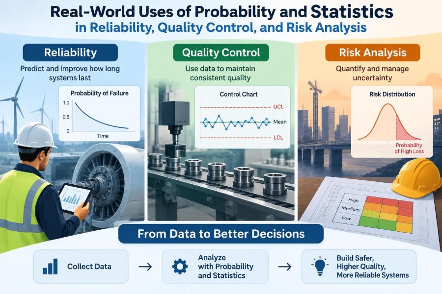
Reliability, quality control, and risk analysis use related mathematical tools, but they ask different practical questions. Understanding the distinction makes probability and statistics much more useful than a collection of formulas.
🎯 Probability Turns Uncertainty into a Usable Quantity
Probability describes how likely an event is within a defined model or set of conditions. A probability of 0 means the event cannot occur in that model, while 1 means it is certain. Most engineering questions live between those limits.
For example, a component may have a small probability of failing during a specified operating period. That number is meaningful only when the component type, loading, environment, and time interval are clear. Saying a pump is “unlikely to fail” is far less useful than defining the conditions under which failure was assessed.
Probability does not predict the fate of one individual unit with certainty. It supports better decisions across many units, repeated operations, or credible future scenarios.
📊 Statistics Extracts Evidence from Measurements
Statistics is the discipline of collecting, summarising, and interpreting data. Engineers use it when measurements are variable: dimensions from a machine, battery lifetimes, vibration readings, test strengths, or delivery times.
A mean gives a central value, but it does not show the full story. Two production processes can have the same average shaft diameter while one produces a much wider spread. That wider spread may create assemblies that bind or rattle even though the average dimension looks correct.
Statistical analysis therefore asks both “What is typical?” and “How much does it vary?” In reliability and quality work, the second question is often the one that reveals a future problem.
🔗 Why Reliability, Quality, and Risk Belong Together
Reliability concerns whether an item performs its required function for a stated time and under stated conditions. Quality control concerns whether a process or product consistently meets requirements. Risk analysis combines the likelihood of an unwanted event with its consequences.
These areas overlap. A machining process with excessive variation can produce a weak part; the weak part can reduce system reliability; its failure may create a safety, financial, or environmental risk. The same measurements can therefore inform all three decisions.
The emphasis changes with the question. Quality teams may focus on reducing variation today, reliability engineers on performance over time, and risk teams on prioritising the most serious failure scenarios.
🧩 Defining the Event Before Doing the Mathematics
Useful analysis begins with an exact event definition. “Failure” could mean a motor stops, its speed drops below a limit, its temperature exceeds a threshold, or it needs maintenance. These are different events and can have different probabilities.
Engineers should also specify exposure: number of operating cycles, kilometres travelled, hours at load, or production units made. A defect rate per thousand parts cannot be compared directly with a failure rate per operating hour.
Clear definitions prevent a common mistake: calculating a precise number for an ambiguous question. Precision in arithmetic cannot repair vagueness in the engineering requirement.
🪙 Random Variables Model What Can Change
A random variable assigns a numerical value to an uncertain outcome. It might be the lifetime of a bearing, the number of defects in a batch, peak wind speed, or the force needed to break a specimen.
Some variables are discrete, such as the number of rejected circuit boards. Others are continuous, such as thickness or time to failure. The distinction influences which probability models and calculations make sense.
Choosing a random variable is an engineering choice, not merely a mathematical one. If the practical concern is a seal leaking, elapsed time until leakage may be more informative than a broad and poorly defined “condition score.”
📈 Distributions Describe Patterns, Not Just Averages
A probability distribution describes which values are common, rare, or extreme. The normal distribution is familiar because many measurements cluster around a mean, but it is not a universal default.
Failure times often have a skewed distribution: they cannot be negative, and a small number of units may survive much longer than the rest. Counts of rare defects may be better represented by discrete models. Engineers should select a distribution from physical understanding and data checks rather than convenience.
Plotting a histogram, probability plot, or empirical cumulative distribution is often a sensible first step. A model that looks elegant but misrepresents the tails can underestimate the events that matter most.
⏳ Reliability Is a Probability Over Time
Reliability is commonly written as R(t) = P(T > t), where T is time to failure. In words, it is the probability that an item survives beyond time t.
A reliability requirement is incomplete without the mission time and operating conditions. A valve can be highly reliable for a short emergency operation yet unsuitable for years of continuous cycling. Temperature, contamination, vibration, duty cycle, and maintenance policy all affect the relevant probability.
This time-based view explains why a successful factory acceptance test does not automatically demonstrate long-term reliability. It verifies something valuable, but only over the conditions and duration actually tested.
🦇 The Bathtub Curve Explains Changing Failure Behaviour
Many products show a broad pattern called the bathtub curve, named for the shape of failure rate over time. The early period may contain infant failures caused by manufacturing defects, installation errors, or weak components. A middle period may have a relatively stable random failure rate, followed by a wear-out period as ageing mechanisms dominate.
This is a conceptual pattern, not a law that every product must follow. Still, it helps separate problems requiring different actions: screening or process improvement for early failures, design robustness for random failures, and planned replacement or condition monitoring for wear-out.
⚙️ Failure Rate Is Not the Same as Failure Probability
The failure rate, often called hazard rate, describes the instantaneous tendency to fail among units that have survived so far. It is not simply the percentage that has failed.
A constant hazard rate can lead to an exponential reliability model, written R(t) = e-λt in conventional notation, where λ is the rate parameter. This model is useful in some situations, but assuming it blindly can hide ageing or early-life effects.
A rising hazard rate suggests wear-out; a falling one may indicate early defects being removed from the population. Maintenance plans should respond to the failure mechanism, not just to a single summary rate.
🛠️ Maintainability Changes System Availability
A reliable item fails infrequently, but a maintainable item can be restored quickly and safely. The practical service measure is often availability: the proportion of time a system is able to perform its intended function.
For equipment with repairable failures, downtime depends on diagnosis, access, spare parts, labour, testing, and restart procedures. Improving mean time to repair can raise availability even when the underlying failure frequency remains unchanged.
This matters in facilities such as data centres, factories, and transport networks. A component that is slightly less durable but easy to replace may sometimes be a better system choice than a highly durable component with a long, complex repair process.
🧱 Series and Parallel Systems Have Different Weak Points
In a series system, every required element must work. If any essential element fails, the system function is lost. A simple model for independent components multiplies their reliabilities, so adding essential parts can reduce overall reliability.
In a parallel system, redundant paths can perform the function. Backup pumps, dual power supplies, and duplicated sensors are examples. Redundancy can improve reliability, but only if failures are sufficiently independent and switching works when needed.
Designers must identify the actual functional architecture. Two components installed side by side are not automatically redundant if one shared controller, cable, power source, or environment can disable both.
🌩️ Common-Cause Failures Can Defeat Redundancy
A common-cause failure occurs when a shared cause disables multiple components. Flooding can affect two generators in the same room; a software defect can affect identical controllers; contaminated fuel can stop several engines.
This is why independent-looking reliability calculations may be overly optimistic. Multiplying probabilities assumes a degree of independence that must be justified. Physical separation, design diversity, separate power feeds, and independent testing can reduce common causes.
Redundancy is therefore not simply “add another unit.” It is a design strategy that must account for shared dependencies.
🏭 Quality Control Looks for Process Stability
Quality control asks whether a process is behaving predictably enough to meet its requirements. A stable process still has natural variation, sometimes called common-cause variation. An unstable process has additional assignable causes, such as a worn tool, incorrect setup, material change, or sensor problem.
The goal is not to inspect defects into submission. It is to understand and control the process that creates the product. When variation is reduced at the source, fewer parts need sorting, rework, or disposal.
That shift from detection to prevention is one of the most practical uses of statistics in manufacturing.
📉 Control Charts Separate Signal from Routine Noise
A control chart plots a process measurement or statistic over time with a centre line and statistically chosen control limits. It helps teams distinguish normal short-term variation from patterns that warrant investigation.
For example, a run of measurements on one side of the centre line, a sudden shift, or a point beyond a limit can indicate that the process changed. The response should be to investigate a cause, not automatically to adjust the machine after every small fluctuation.
Over-adjustment, often called tampering, can make a stable process worse. Control charts provide disciplined evidence for when intervention is justified.
📏 Specification Limits and Control Limits Answer Different Questions
These limits are often confused. Specification limits come from the product requirement: the acceptable range for a dimension, strength, or performance measure. Control limits are calculated from process behaviour and indicate whether the process appears stable.
| Limit type | Primary question | Set by |
|---|---|---|
| Specification limit | Does the product meet its requirement? | Design, customer, or regulatory requirement |
| Control limit | Is the process behaving consistently? | Statistical analysis of process data |
A process can be statistically stable but consistently produce items outside specification. It can also be unstable while the latest items happen to meet specification. Both conditions require attention, but for different reasons.
🎯 Process Capability Connects Variation to Tolerance
Process capability assesses whether a stable process has enough room within specification limits. It compares the process spread and centring with the permitted tolerance.
Capability indices such as Cp and Cpk are widely used, but their interpretation requires care. They rely on assumptions about stability, measurement quality, and the distribution of data. A high index based on a short or unrepresentative sample can create false confidence.
Before celebrating a capability result, confirm that the process is under control and that the measurement system can resolve the variation being assessed.
🔍 Measurement Systems Can Hide or Create Variation
No quality decision is stronger than the measurement behind it. A gauge may have bias, poor repeatability, poor reproducibility between operators, limited resolution, or drift over time.
Imagine measuring a tight diameter tolerance with an instrument whose readings fluctuate almost as much as the parts themselves. The observed spread then mixes true product variation with measurement noise. Decisions about capability, supplier performance, or machine adjustment become unreliable.
Gauge studies, calibration, clear work instructions, and appropriate sampling conditions help ensure that data describes the product rather than the instrument’s limitations.
🎲 Sampling Inspection Balances Information and Cost
Inspecting every unit can be justified for critical characteristics or automated high-speed checks, but it is not always practical or even destructive-test compatible. Acceptance sampling uses a sample from a lot to decide whether the lot meets an agreed rule.
Sampling carries two unavoidable risks: accepting a poor lot or rejecting a good lot. The plan controls these risks rather than eliminating them. Larger samples generally provide more information, but they cost more time and resources.
Sampling is best treated as a decision tool, not proof that every accepted item is defect-free. Process control upstream remains the stronger long-term quality strategy.
🧪 Accelerated Testing Reveals Weaknesses Faster
Reliability tests can take too long if products normally operate for years. Accelerated testing uses elevated stress, such as temperature, cycling rate, voltage, humidity, or load, to expose failure mechanisms more quickly.
The critical condition is relevance. A test is useful when the added stress accelerates the same mechanism expected in normal service. Excessive or unrealistic stress can create failures that would not occur in the field, leading to misleading conclusions.
Engineers need a physically credible relationship between test conditions and use conditions before extrapolating accelerated results to service life.
🧭 Risk Combines Likelihood, Consequence, and Exposure
Risk is often described as a combination of likelihood and consequence. In practice, exposure also matters: a hazard encountered frequently can deserve attention even if each individual encounter is unlikely to cause harm.
A minor production defect may be economically important when it occurs across a large volume. Conversely, a very rare event with severe consequences may justify strong controls despite limited historical data. Risk analysis helps compare unlike problems on a structured basis.
Numbers support judgement; they do not replace it. Consequences can include injury, service disruption, environmental harm, lost data, repair cost, and reputational effects, not just one monetary value.
🗺️ Risk Matrices Are Useful, but Coarse
A risk matrix places likelihood and consequence into categories such as low, medium, or high. It is easy to communicate and can help teams prioritise discussions, especially early in a project.
Its limitation is that categories compress detail. Two risks placed in the same cell may have very different mechanisms, uncertainty, detectability, or control options. Boundary choices can also change the displayed priority.
Use a matrix as a conversation and screening tool, then investigate significant hazards with more detailed evidence, scenarios, or quantitative models where the decision warrants it.
🌳 Fault Trees Trace How Top Events Can Happen
A fault tree analysis starts with an unwanted top event, such as loss of braking or failure to cool a process, and works backward through logical causes. AND gates require several events together; OR gates mean any one input can cause the event.
The method reveals combinations that may be missed by a simple checklist. It also highlights single points of failure and shared dependencies. Where suitable probability data exists, the tree can support a quantitative estimate.
The quality of a fault tree depends on its scope and assumptions. It is not a substitute for understanding the physical system, operating procedures, human interactions, and external hazards.
🧠 FMEA Starts with Failure Modes and Effects
Failure modes and effects analysis, or FMEA, examines how each item or process step might fail, what effect that failure would have, and how it can be detected or prevented. It is especially useful early in design and process planning.
Teams often record severity, occurrence, and detection ratings. These ratings can organise discussion, but multiplying subjective scores into one priority number should not obscure a serious hazard. A high-severity failure deserves explicit attention even when it is believed to be uncommon.
A valuable FMEA ends with owners, actions, and follow-up evidence. A spreadsheet full of ratings without changes to the design or process is not risk reduction.
📚 Bayesian Updating Lets Evidence Refine a Prior View
Bayesian reasoning combines prior knowledge with new evidence. A prior estimate might come from similar equipment, engineering judgement, or earlier tests. New inspection results or field observations then update that estimate.
This is particularly helpful when data is limited, which is common for novel systems and rare failures. It makes assumptions visible rather than pretending that a small dataset speaks entirely for itself.
The result still depends on the quality of the prior and the relevance of the new data. Bayesian methods are not a shortcut around weak evidence; they are a structured way to use incomplete evidence honestly.
📦 Spare Parts and Inventory Decisions Use Demand Uncertainty
Maintenance teams must decide how many critical spares to hold. Too few can extend downtime; too many tie up capital, storage space, and may create obsolescence problems. Failure demand is uncertain, so average demand alone is not enough.
Useful inputs include expected failure behaviour, repair lead time, usage variability, the ability to borrow or substitute parts, and the consequence of a stockout. A rare part with a long lead time and severe downtime consequence may deserve stocking even when its average annual demand is low.
Statistics turns this from guesswork into an explicit service-level and risk trade-off.
📡 Condition Monitoring Supports Decisions Before Failure
Condition monitoring uses signals such as vibration, temperature, lubricant debris, acoustic emissions, or electrical signatures to detect deterioration. The objective is not merely to collect more data; it is to identify a condition change early enough to act.
Thresholds should reflect both false alarms and missed detections. An overly sensitive alarm sends teams chasing harmless noise, while an insensitive alarm provides warning only when repair options are limited.
Trend analysis can be more useful than one reading. A vibration level that remains steady may be normal for a specific machine, while a sustained upward trend under comparable load can signal a developing fault.
⚠️ Rare Events Need More Than Historical Frequencies
For rare, high-consequence events, historical data may contain few or no examples. Zero observed failures in a limited period does not prove zero risk; it may simply mean the observation window was too small or conditions were not challenging enough.
Engineers can combine available data with physics, design review, scenario analysis, near-miss reports, and conservative assumptions. Uncertainty should be documented, especially when decisions depend heavily on extrapolation.
This is not an argument for treating every remote scenario as equally likely. It is an argument for avoiding the opposite mistake: dismissing a credible hazard only because the past record is sparse.
🧹 Data Quality Determines Model Quality
Incorrect timestamps, missing operating hours, inconsistent failure codes, changed sensor calibrations, and unrecorded maintenance can distort an analysis. A sophisticated model fitted to poor data may appear convincing while producing unreliable recommendations.
Good practice includes defining failure codes, recording exposure as well as failures, preserving configuration history, and checking for censored data. A unit removed from a study before it fails contributes information, but it should not be treated as if its lifetime were known.
Data governance may feel administrative, yet it is a technical control. It determines whether future teams can learn from current operations.
🚫 Common Statistical Mistakes in Engineering Decisions
Several errors recur because they produce simple answers quickly:
- Using an average while ignoring spread, skewness, or extreme values.
- Assuming independence between failures that share power, software, environment, or operators.
- Confusing correlation with causation when two variables move together.
- Declaring a process capable before checking stability and measurement adequacy.
- Using a probability model outside the operating conditions from which it was estimated.
- Treating a risk ranking as an objective fact rather than a structured judgement with assumptions.
The remedy is not mathematical perfection. It is transparent assumptions, sensible visual checks, engineering review, and willingness to revise a model when the system changes.
🤝 Communication Makes Quantitative Analysis Actionable
A probability estimate is useful only if decision-makers understand what it means, what it does not mean, and what action follows. “One percent risk” is incomplete without a time period, population, consequence, uncertainty range, and comparison with alternatives.
Visuals, plain language, and scenario descriptions help. Instead of reporting only a failure rate, explain the likely maintenance burden, expected downtime exposure, key drivers, and the conditions that could invalidate the estimate.
Clear communication also prevents a dangerous misunderstanding: low probability does not necessarily mean low priority when consequences are severe.
🧭 A Practical Workflow for Better Decisions
A sound analysis does not need to start with complex software. It starts with a disciplined sequence:
- Define the function, failure event, time horizon, and operating conditions.
- Map failure mechanisms, process steps, dependencies, and consequences.
- Check whether measurements and records are fit for purpose.
- Use descriptive statistics and plots before fitting advanced models.
- Select models whose assumptions match the engineering situation.
- Test sensitivity: ask which uncertain inputs change the decision most.
- Choose controls, owners, thresholds, inspection intervals, or design changes.
- Monitor results and update the analysis when new evidence arrives.
This loop connects mathematics to learning. A model is not the final product; a better engineering decision is.
✅ The Core Principle: Manage Variation and Uncertainty Deliberately
Probability and statistics are valuable because engineering systems are variable, interconnected, and exposed to incomplete information. Reliability analysis asks whether a function will endure, quality control asks whether a process stays within requirements, and risk analysis asks which uncertain outcomes deserve the strongest controls.
The best results come from combining data with physical understanding. Models should state their assumptions, measurement systems should be questioned, and rare but credible scenarios should not disappear simply because they are inconvenient to quantify.
Used this way, engineering mathematics does not promise certainty. It provides a disciplined basis for designing safer systems, producing more consistent work, and making trade-offs visible before failures make them for us.
The practical value of probability and statistics is not predicting every outcome; it is making uncertainty measurable enough to manage wisely. 📐📊⚙️