
When wind bends trees, water moves through a pipe, or a motor turns a conveyor belt, something is changing from place to place. The change is not only about “how much.” Direction matters too.
An engineer designing a ventilation system needs to know where air is moving, how fast it is moving, and whether it swirls near a corner. A structural engineer needs to understand forces at many points in a beam. An electrical engineer needs a map of the electric and magnetic influence around a device.
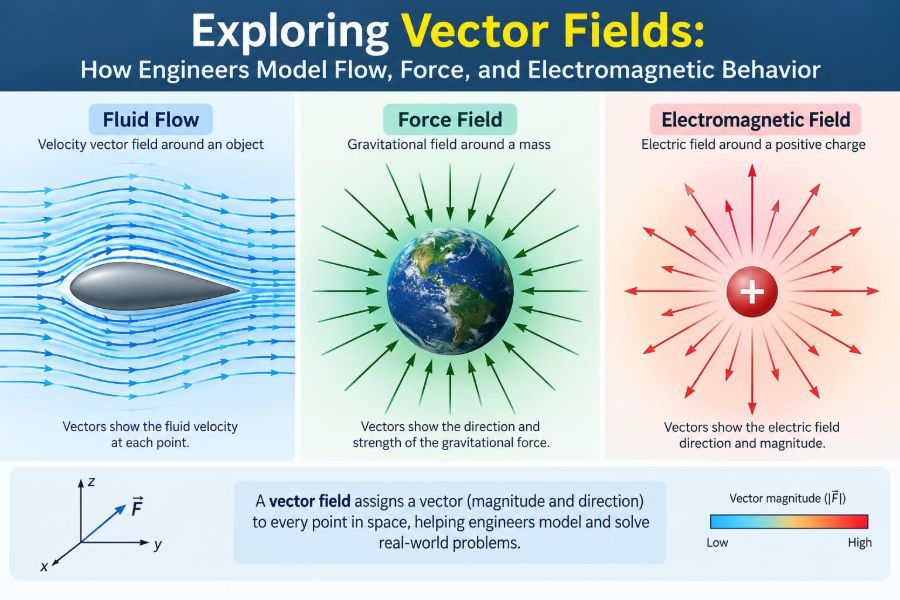
These situations can look unrelated, but mathematics gives them a common language: the vector field. It assigns a vector—an amount with direction—to every relevant point in space and, sometimes, time.
Vector fields turn an invisible pattern into something that can be calculated, visualized, and tested. They are central to fluid mechanics, mechanics, electromagnetics, heat transfer, control, and simulation.
🧭 What a Vector Field Represents
A scalar field assigns one number to each location. Temperature in a room is a familiar example: every point has a temperature, but temperature itself does not point in a direction.
A vector field assigns a vector at each location. In three dimensions, it is commonly written as F(x,y,z) = P(x,y,z)i + Q(x,y,z)j + R(x,y,z)k. The components describe the field’s strength along the coordinate directions.
For a velocity field, the vector tells us the local direction and speed of motion. For a force field, it tells us the force a suitable object would experience at that point.
📍 Why “At Every Point” Changes the Problem
A single vector can describe one push or one velocity. A vector field describes a whole region. That distinction matters because engineering systems rarely behave identically everywhere.
Water near the center of a pipe usually moves differently from water near its wall. Magnetic influence varies around a current-carrying conductor. A field captures these local differences without reducing the system to one average value.
The field is a model, not the physical object itself. Its value depends on what quantity is being modeled and on the assumptions used to build the model.
➡️ Reading Arrows in a Field Plot
The most direct visualization is a vector plot, sometimes called a quiver plot. An arrow is placed at selected locations: its orientation indicates direction, while its length or color indicates magnitude.
Long arrows are not automatically “more dangerous” or “better.” They only mean the modeled quantity is larger under the chosen scale. Plotting software often rescales arrows so that crowded diagrams remain readable.
When reading a plot, first check the legend, coordinate axes, units, and scaling convention. A visually persuasive diagram can still be misleading if its magnitudes are normalized or its sampling is sparse.
📏 Magnitude, Direction, and Components
For a vector F = Pi + Qj + Rk, its magnitude is |F| = sqrt(P² + Q² + R²). This is the local size of the vector, such as speed in a velocity field.
Components are equally useful because engineering constraints are often directional. A wind load’s horizontal component may control drift, while its vertical component may affect uplift. A robot arm may need force in one direction while limiting force in another.
Separating components also makes equations manageable. The physical meaning should not disappear, however: each component is tied to a chosen coordinate system and its directions.
🗺️ Scalar Fields and Vector Fields Work Together
Many systems require both kinds of fields. In fluid flow, pressure is commonly modeled as a scalar field, while velocity is a vector field. In heat transfer, temperature is scalar, while heat flux—the direction and rate of heat flow per area—is vector-valued.
| Quantity | Field type | Typical engineering question |
|---|---|---|
| Temperature | Scalar | Where is the component hottest? |
| Fluid velocity | Vector | Where and how fast is fluid moving? |
| Pressure | Scalar | How does loading vary across a surface? |
| Electric field | Vector | What force direction acts on a charge? |
| Heat flux | Vector | Where is thermal energy flowing? |
Understanding which quantity is scalar and which is vector prevents a common error: treating a directional transport process as if only its size mattered.
🌊 Velocity Fields Describe Fluid Motion
A velocity field may be written as v(x,y,z,t). The extra variable t means the flow can change with time, as it does when a pump starts, a valve closes, or wind gusts pass a building.
Imagine dye released into a channel. The dye does not create the velocity field; it reveals how the field transports material. Its path can expose fast central flow, slow boundary regions, recirculation zones, and mixing patterns.
Engineers use velocity fields to assess pressure loss, cooling performance, pollutant dispersion, pump selection, and the movement of particles or droplets.
🚰 The Pipe-Flow Example
In an idealized straight pipe, flow is often mainly axial: velocity points along the pipe’s length. Yet the magnitude can vary across the radius. Fluid near a stationary wall is slowed by viscosity, the fluid property that resists relative motion.
For steady laminar flow in a circular pipe, an ideal model gives a smooth, parabolic speed profile: greatest at the center and zero at the wall. Real systems may depart from this picture because of roughness, bends, fittings, turbulence, or changing flow rate.
This profile matters when estimating wall shear, residence time, heat transfer, and whether a sensor placed at one point represents the average flow.
🌀 Streamlines, Pathlines, and Streaklines
These terms are often used loosely, but they answer different questions. A streamline is a curve tangent to the instantaneous velocity field; at one selected time, it shows the local direction of flow.
A pathline is the route followed by one individual particle over time. A streakline is the collection of particles that have passed through a fixed release point, such as continuous smoke from a nozzle.
In steady flow, the three coincide. In unsteady flow, they can differ substantially, which matters when interpreting flow-visualization experiments or animation results.
🔄 Circulation Reveals Swirling Motion
Circulation measures how strongly a vector field tends to follow a closed loop. Mathematically, it is evaluated with a line integral around that loop.
A paddle wheel placed in a flow gives a useful intuition. If the wheel spins, the nearby field has local rotational behavior. A swirling drain, a mixing tank, and airflow near a rotating fan can all show this effect.
Circulation depends on the chosen loop, so it is not simply a label of “vortex present” or “vortex absent.” The loop’s size, position, and orientation affect the result.
🧲 Curl Measures Local Rotation
The curl of a vector field is another vector field, written ∇ × F. It measures local rotational tendency rather than motion around one particular large loop.
For a velocity field, curl is closely related to vorticity. Its direction follows the right-hand rule, and its magnitude indicates the local strength of rotation under the field’s units.
Zero curl does not mean that nothing moves. A uniform wind can have nonzero velocity everywhere while having zero curl, because neighboring parts of the flow do not rotate relative to one another.
💨 Divergence Measures Net Outflow
The divergence, written ∇ · F, is a scalar that measures the net outward flow per unit volume near a point. Picture a tiny closed box placed in a field: divergence compares what leaves the box with what enters.
Positive divergence suggests net outward behavior, while negative divergence suggests net inward behavior. In a velocity field, the interpretation depends on the physical model and whether material can be compressed.
Divergence is local. Arrows spreading apart in a drawing can be suggestive, but the actual value comes from how the field changes in all coordinate directions.
🫧 Incompressible Flow and Continuity
For an incompressible fluid with constant density, the continuity equation commonly reduces to ∇ · v = 0. This says that fluid is not accumulating or disappearing within a tiny fixed volume.
It does not say the velocity is constant. When water enters a narrower section of a pipe, its speed can increase while the divergence remains zero. The geometry redirects and redistributes the velocity field.
Air is often approximated as incompressible at relatively low speeds and modest pressure changes, but that approximation has limits. Compressibility becomes significant in many high-speed or strongly pressure-varying applications.
🧱 Force Fields Turn Location into Loading
A force field assigns the force on a specified object or property at each position. Gravitational fields, electric fields, and magnetic effects are common examples, though the precise force law depends on the object involved.
Near Earth’s surface, gravitational acceleration is often approximated as a nearly uniform downward field for local engineering calculations. Over larger distances or precision-sensitive problems, its direction and magnitude vary with position.
Distributed mechanical loading also has a field-like character. Pressure on a dam wall varies across the surface; body force in a solid acts throughout its volume.
🪂 Potential Energy and Conservative Fields
Some force fields are conservative. In such a field, work done moving between two points does not depend on the path taken; it depends only on the endpoints. Gravity in a simplified static setting is a familiar example.
A conservative field can be derived from a scalar potential. In one common sign convention, F = -∇V, where V is potential energy per appropriate unit.
This relationship is powerful because it converts a vector problem into changes in one scalar quantity. It does not apply to every force. Friction, for example, generally depends on the path length and dissipates mechanical energy.
⛰️ The Gradient Points Uphill
The gradient of a scalar field, written ∇φ, is a vector pointing in the direction of the steepest local increase of φ. Its magnitude gives the rate of that maximum increase per unit distance.
On a topographic map, the gradient of elevation points uphill and is perpendicular to contour lines. For temperature, the gradient points toward warmer conditions, not necessarily toward heat flow.
This distinction is essential: heat flux in ordinary conduction is commonly modeled as pointing opposite the temperature gradient. Thermal energy flows from warmer to cooler regions.
🔥 Heat Flux Is a Directional Transport Field
Fourier’s law for simple conduction is often written as q = -k∇T, where q is heat flux, k is thermal conductivity, and T is temperature. The minus sign expresses the familiar hot-to-cold direction.
In isotropic materials, conductivity behaves like a scalar. In some engineered or naturally structured materials, conductivity can be direction-dependent, requiring a more advanced tensor description rather than one number.
Thermal field plots help identify hot spots, insulation weaknesses, and paths of unwanted heat loss. They must be interpreted alongside boundary conditions, material data, and the model’s assumptions.
⚡ Electric Fields and Electric Force
An electric field E gives the force per unit positive test charge at a location. The force on a charge q is modeled by F = qE in a simple electrostatic context.
Field lines are a visualization device: their tangent direction follows the electric field, and denser line drawings are often used to suggest stronger magnitude. They are not physical threads traveling through space.
Engineers use electric-field analysis when designing insulation, capacitors, sensors, high-voltage equipment, printed circuit layouts, and devices where concentrated fields can trigger unwanted discharge or material stress.
🧲 Magnetic Fields Depend on Motion and Geometry
Magnetic fields are vector fields, but their force effects differ from electric fields. A moving charge experiences magnetic force according to F = q(v × B), where v is velocity and B is magnetic flux density.
The cross product means the magnetic force is perpendicular to both motion and field direction. Consequently, an ideal magnetic field can bend a charged particle’s path without directly changing its speed.
Motors, generators, inductors, imaging instruments, and many sensors rely on carefully shaped magnetic fields. Geometry, material properties, and time-varying currents all influence the result.
🔌 Maxwell’s Equations Connect the Fields
Maxwell’s equations provide a compact framework linking electric and magnetic behavior. In differential form, they relate divergence and curl to charge, current, and time-varying fields.
One key idea is mutual coupling: changing magnetic fields can produce electric fields, and changing electric fields contribute to magnetic fields. This is the foundation of electromagnetic induction and electromagnetic waves.
Practical electromagnetic models may also need material constitutive relations, losses, boundary conditions, and frequency-dependent properties. The compact equations are powerful, but applying them correctly requires a complete physical model.
🧮 Differential Operators Extract Useful Behavior
The symbol ∇, pronounced “del,” packages spatial derivatives. Applied in different ways, it produces several central operations:
- Gradient:
∇φ, turning a scalar field into a vector field. - Divergence:
∇ · F, measuring local net outflow. - Curl:
∇ × F, measuring local rotational tendency. - Laplacian:
∇²φ, describing local curvature-like variation in many diffusion and potential equations.
These are not merely symbolic operations. Each answers a different physical question, so choosing the wrong one can produce an equation with no meaningful interpretation.
🧭 Coordinate Systems Should Match the Geometry
Cartesian coordinates suit rectangular ducts, plates, and many structural components. Cylindrical coordinates often simplify pipes, shafts, and rotating machines. Spherical coordinates are useful for radially symmetric fields.
The field itself is independent of the coordinate system, but its components and equations change with the basis. In curvilinear coordinates, unit directions can vary from point to point, so derivative formulas require additional geometric terms.
A common student mistake is to use Cartesian divergence or curl formulas unchanged in cylindrical geometry. Select the coordinate system first, then use the operator form appropriate to it.
🧩 Boundary Conditions Complete the Model
Field equations alone rarely determine a unique engineering solution. Boundary conditions specify what happens at edges, surfaces, or interfaces: a fixed temperature, prescribed flow speed, known voltage, applied traction, or insulation condition.
Initial conditions are also required for time-dependent problems. They define the field at the starting time, after which the governing equations describe its evolution.
Small changes in boundaries can strongly alter a field. A sharp electrode, blocked vent, wall roughness, or imperfect thermal contact can create concentrated gradients that a simplified model may miss.
🧱 Interfaces Create Changes in Field Behavior
At an interface between materials, fields typically obey continuity or jump conditions derived from conservation laws and constitutive behavior. The exact conditions depend on the phenomenon being modeled.
For example, heat flux normal to a well-bonded interface is commonly continuous in steady conduction, while the temperature gradient can change because the materials have different conductivities. In electromagnetics, material permittivity and permeability affect how fields distribute across interfaces.
These effects explain why field maps often bend, concentrate, or change slope at material boundaries. Ignoring interfaces can make a model look smooth while missing the location most likely to govern performance.
🧱 Discretization Turns Fields into Computation
Analytical solutions are valuable, but real geometries and operating conditions often require numerical methods. Finite difference, finite volume, and finite element methods replace a continuous field with values over a mesh or grid.
The governing equations are approximated by algebraic equations, then solved computationally. A finer mesh can capture sharper variation, but it also increases computational cost and does not automatically guarantee accuracy.
Mesh quality matters especially near walls, corners, thin layers, and field singularities. The numerical result should be treated as an approximation that needs checking, not as a picture that is correct because software produced it.
✅ Verification and Validation Are Different Checks
Verification asks whether the mathematical model and numerical implementation were solved correctly. Typical checks include mesh refinement, dimensional consistency, conservation balance, and comparison with a case that has a known solution.
Validation asks whether the model represents the physical system adequately for its intended use. This can involve comparison with suitable measurements, while recognizing uncertainty in sensors, material properties, operating conditions, and geometry.
A calculation can be verified yet not validated if its assumptions omit an important physical effect. Conversely, agreement with one measurement does not establish that a model will predict every operating condition accurately.
📊 Field Measurements Need Spatial Awareness
Measurements of a field are sampled, not continuous. A pressure tap reports conditions at a location; a thermocouple has finite size; a velocity probe can disturb sensitive flows; magnetic sensors have orientation and bandwidth limits.
Interpolation between measurements may be useful, but it introduces assumptions about how the field varies. Sparse sampling can miss peaks near sharp corners, interfaces, and boundary layers.
When comparing measurements with simulation, match the reported quantity carefully. A sensor may measure an average over its sensing volume or over time, rather than the exact point value displayed in a numerical model.
⚠️ Common Interpretation Mistakes
Several errors recur when field concepts are learned only as formulas:
- Confusing a field line with the actual path of a particle in unsteady flow.
- Assuming zero divergence means zero velocity.
- Assuming zero curl means a field has no motion or no influence.
- Ignoring units when combining field quantities and derivatives.
- Treating an arrow diagram as quantitative without checking its scale.
- Using a point value as if it represented an entire cross-section or volume.
Each mistake comes from losing the connection between the mathematics and the physical question. Naming the quantity, region, coordinate system, and units before calculating is an effective safeguard.
🛠️ A Practical Workflow for Field Problems
Start by stating what field is needed and what its units mean. Then identify the domain, coordinate system, relevant conservation law, material model, and boundary or initial conditions.
- Sketch the geometry and mark expected directions of flow, force, or transport.
- Choose a suitable field variable, such as velocity, temperature, electric potential, or flux.
- Write the governing relationship and list assumptions explicitly.
- Estimate scales to check whether simplifications are reasonable.
- Solve analytically or numerically, then test conservation and limiting cases.
- Interpret the field in terms of a design decision, not only a contour plot.
This workflow makes it easier to notice when a polished result rests on weak inputs or an inappropriate approximation.
🏭 Where Engineers Use Vector Fields Every Day
In aerospace, velocity and pressure fields help assess lift, drag, cooling, and plume behavior. In civil engineering, wind, groundwater, stress, and heat fields inform building and infrastructure design.
Mechanical engineers work with stress-related vector and tensor quantities, lubricant flow, thermal flux, and magnetic actuator fields. Electrical engineers model electric and magnetic fields for power systems, antennas, motors, and electronic packaging.
Environmental and biomedical applications also depend on field reasoning: dispersion in air and water, blood flow, diffusion, and transport through porous materials. The mathematical framework transfers because the underlying question is similar—how does a quantity vary across space?
🎯 The Core Idea: Local Direction Creates System Behavior
Vector fields are valuable because complex engineering behavior emerges from local information. At each point, a vector says what direction a quantity acts or moves and how strongly. Across a region, those vectors reveal patterns such as transport, rotation, accumulation, and concentration.
Gradient, divergence, and curl provide complementary ways to interrogate those patterns. Boundary conditions and material properties then determine how the field is constrained in a real device or environment.
The most useful habit is to move back and forth between picture, equation, and physical meaning. A field plot should prompt questions: What does each arrow represent? What creates this pattern? What design consequence follows from it?
Vector fields give engineers a disciplined way to convert spatial variation into predictions about flow, force, energy, and electromagnetic behavior. Once that connection is clear, equations become less abstract and far more useful in design and problem-solving. 📐🌊⚡