
A robot arm reaches for a component on an assembly line. A control system corrects a drone drifting sideways. An engineer adjusts the parameters of a thermal model until its predicted temperatures match measured data.
These tasks look different, but each depends on the same practical question: if one input changes slightly, what happens to every output? A Jacobian matrix is a compact mathematical answer to that question.
It turns a complicated nonlinear relationship into a local, usable map of change. That map helps engineers predict motion, choose corrections, estimate unknown parameters, and recognize when a model or mechanism is close to a troublesome configuration.
Once Jacobians are seen as “sensitivity maps,” rather than as a page of partial derivatives, their role in robotics, optimization, and engineering analysis becomes much easier to understand.
🧭 The Core Idea: A Map of Local Change
Suppose a system has several inputs and several outputs. Inputs might be motor angles, material properties, voltages, or design dimensions. Outputs might be position, force, temperature, cost, or error.
A Jacobian matrix records how each output responds to a small change in each input at a particular operating point. It is a local description: it is reliable for nearby changes, not automatically for large jumps across a nonlinear system.
📦 From Ordinary Derivatives to Many Variables
For a one-variable function, a derivative is a slope. If y = f(x), then dy/dx describes the approximate change in y caused by a small change in x.
Engineering systems rarely have only one input and one output. If a function produces an output vector y from an input vector x, its Jacobian extends the familiar derivative to this multivariable setting.
🧮 Reading the Jacobian Matrix
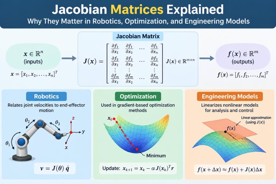
Let f: Rⁿ → Rᵐ, meaning that n inputs produce m outputs. The Jacobian is written as J and has m rows and n columns.
J = [∂fᵢ/∂xⱼ]
Entry ∂fᵢ/∂xⱼ means: how does output i change when input j changes, while the other inputs are held fixed? Rows correspond to outputs; columns correspond to inputs.
🔍 A Small Two-Input Example
Consider the hypothetical mapping f(x, y) = [x²y, x + 3y]. It has two inputs and two outputs, so its Jacobian is a 2 × 2 matrix:
J(x,y) = [2xy   x²]
         [ 1     3]
At (x, y) = (1, 2), the Jacobian becomes [[4,1],[1,3]]. For example, the upper-left value says that a small increase in x changes the first output by approximately four times that increment at this specific point.
📍 Why the Operating Point Changes Everything
In a linear system, sensitivities are constant. In nonlinear systems, they vary with state. The Jacobian for a robot arm differs when the arm is folded versus extended, just as the sensitivity of heat transfer can differ at different temperatures.
This is why engineers evaluate a Jacobian at an operating point. A matrix calculated at one state should not be assumed valid everywhere else.
📏 Linearization: Turning Curves into Local Planes
The central approximation is:
f(x + Δx) ≈ f(x) + J(x)Δx
This says that a small output change Δf can be estimated by multiplying the Jacobian by a small input change Δx. Geometrically, a curved relationship is replaced nearby by its tangent line, tangent plane, or higher-dimensional equivalent.
Linearization does not remove the system’s nonlinearity. It provides a manageable local model that can be recalculated as the state changes.
🛠️ Units Give Each Entry Physical Meaning
Jacobian entries carry units. If a robot’s output is measured in metres and its joint angle in radians, the relevant entry has units of metres per radian. If an output is voltage and an input is temperature, an entry may be volts per degree.
Checking units is a simple but powerful error check. It also reveals why scaling matters: a matrix mixing millimetres, metres, degrees, and newton-metres may be numerically awkward even when the underlying equations are correct.
🤖 Robot Kinematics: From Joint Motion to Tool Motion
In robot kinematics, the inputs are commonly joint variables, collected in a vector q. The outputs describe the end effector—the gripper, welding torch, or camera—through position and often orientation.
The kinematic Jacobian relates joint velocities to end-effector velocity:
v = J(q)q̇
Here, q̇ is the vector of joint rates and v is a task-space velocity. The matrix says which joint motions contribute to motion in each Cartesian direction and rotational direction.
🦾 A Planar Two-Link Arm
Imagine a two-link arm moving in a flat plane. Its two joint angles determine the horizontal and vertical coordinates of its tip. Differentiating those position equations with respect to both angles gives a 2 × 2 Jacobian.
One column describes the tip velocity caused by moving the first joint alone; the other describes the velocity caused by the second. Since the columns depend on arm geometry and current angles, the same motor speed can create very different tip movements in different poses.
🎯 Inverse Velocity Control
Often the desired quantity is not joint speed but tool speed: “move 2 millimetres per second to the left,” for example. The controller needs to find joint rates that achieve that request.
If the Jacobian is square and invertible, a simple expression is q̇ = J⁻¹v. In practice, robots may have more or fewer joints than task coordinates, so direct inversion is not always possible or desirable.
🚧 Singularities in Mechanisms
A singularity occurs when the Jacobian loses rank. In a planar arm, this can happen when links line up. At that configuration, some tip-motion directions cannot be created independently by small joint changes.
Near a singularity, the calculated joint speeds needed for an ordinary tool motion can become very large. This can exceed actuator limits, magnify measurement noise, and make control feel unstable or erratic.
📉 Rank Explains Lost Directions
Rank counts the number of independent directions represented by a matrix. A full-rank Jacobian provides the expected local freedom; a rank-deficient Jacobian does not.
For a 3D position task, rank three means the end effector can locally generate independent small motions along three directions. Lower rank means that at least one local direction is unavailable or coupled with another.
🧷 Redundancy Creates Useful Freedom
A robot with more controllable joints than task coordinates is redundant. A seven-joint arm positioning a six-dimensional pose is a familiar example. Several joint-velocity choices may produce the same end-effector motion.
This extra freedom can be used to avoid obstacles, stay away from joint limits, reduce energy use, or keep a comfortable working posture. The Jacobian identifies the motions that affect the task and those that lie in its null space.
🧩 The Pseudoinverse When No Ordinary Inverse Exists
The Moore–Penrose pseudoinverse, written J⁺, generalizes inversion for rectangular matrices. A commonly used velocity command is q̇ = J⁺v.
For redundant systems, this often selects a minimum-norm joint velocity among the available solutions. For systems with too few degrees of freedom, it finds a best-fit task velocity under a specified least-squares interpretation. Its behavior near singularities still requires care.
🛡️ Damped Least Squares Near Difficult Poses
Damped least squares modifies the inverse-like calculation to avoid extreme joint rates near singular configurations. A typical form includes a positive damping parameter that reduces amplification of poorly controlled directions.
The trade-off is deliberate: the robot may not exactly achieve the requested instantaneous tool velocity, but it behaves more smoothly and remains within more realistic actuator demands. Damping should be tuned to the application rather than treated as a universal fix.
⚡ Force, Torque, and Virtual Work
The Jacobian also connects forces at a tool to torques at joints:
τ = JᵀF
Here F is an end-effector force or wrench, and τ is the required joint-torque vector. The transpose appears because the relationship preserves virtual work: tool force times a small tool displacement corresponds to joint torque times a small joint displacement.
This relation matters in force control, contact tasks, load estimation, and mechanism design.
📈 Optimization Sees the Jacobian as Sensitivity
Optimization seeks input values that minimize or maximize an objective. When the objective or residuals depend on many parameters, the Jacobian tells an algorithm which parameter adjustments are likely to reduce error locally.
For model fitting, define a residual vector r(x) as the difference between predicted and observed values. Its Jacobian describes how each residual changes with each parameter. That is the information used to choose a corrective step.
🎯 Gauss–Newton for Least-Squares Problems
Many calibration problems minimize the sum of squared residuals, ||r(x)||². Gauss–Newton linearizes the residual vector and solves a local least-squares problem for the parameter update.
The key matrix expression is often written as JᵀJ, where J is the residual Jacobian. It summarizes how parameter changes affect the overall residual pattern. If columns are nearly dependent, the estimation problem may be poorly conditioned.
🧠 Newton’s Method and Second-Order Information
Newton’s method uses gradient and curvature information to update variables. For a scalar objective, the exact curvature is represented by a Hessian matrix, which contains second derivatives.
Jacobians remain central because a gradient itself can be viewed as a Jacobian of a scalar function, and because many practical methods build curvature approximations from residual Jacobians. Gauss–Newton is often attractive when residuals are small or the model is close to a good fit.
🌡️ Parameter Estimation in Engineering Models
Consider a hypothetical heat-transfer model with unknown conductivity and convection parameters. Sensors provide temperatures at several locations. Each residual compares one model prediction with one measurement.
The Jacobian indicates which sensors are sensitive to which parameters. If every measured temperature responds almost identically to two parameters, the data may not be able to distinguish them reliably. This is an identifiability issue, not merely an algorithm failure.
🔌 Circuit and Network Analysis
Nonlinear circuit equations arise from components such as diodes and transistors. To solve them, numerical methods repeatedly linearize the equations around a current voltage estimate.
The Jacobian in this setting is sometimes called a conductance or system matrix at the current iteration. It captures local relationships between node-voltage changes and equation residual changes, enabling a nonlinear network to be solved through a sequence of linear systems.
🌊 Dynamic Systems and State-Space Models
For a nonlinear dynamic model ẋ = f(x,u), engineers form Jacobians with respect to state x and input u. Near a reference state, these become the matrices commonly called A and B:
Δẋ ≈ AΔx + BΔu
This local linear model supports stability analysis, controller design, observer design, and simulation insight. It is only a local approximation, so behavior far from the reference condition can differ substantially.
🛰️ Estimation and the Extended Kalman Filter
The Extended Kalman Filter applies linearization to nonlinear state and measurement models. Their Jacobians propagate uncertainty and determine how strongly new measurements should correct an estimate.
This is useful in navigation, sensor fusion, and tracking, but a poor linearization can cause inaccurate uncertainty estimates or weak convergence. Large nonlinearities, ambiguous measurements, and poor initial conditions call for careful validation or alternative estimation methods.
🧪 Three Ways to Compute a Jacobian
✍️ Analytic differentiation
Deriving partial derivatives by hand gives exact mathematical expressions and often efficient code. The downside is development time and the possibility of algebraic or implementation mistakes in large models.
🔢 Finite differences
Finite differences perturb one input at a time and observe output changes. They are easy to apply to an existing simulation, but the perturbation size matters: too large causes approximation error, while too small can expose numerical roundoff.
⚙️ Automatic differentiation
Automatic differentiation evaluates derivatives through program operations using the chain rule. It is not symbolic algebra and is not ordinary finite differencing. Where supported, it can provide accurate derivatives while reducing manual derivation effort.
🔗 The Chain Rule Builds Large Jacobians
Engineering models are often assembled from stages: geometry feeds physics, physics feeds sensors, and sensors feed an objective. If y = g(z) and z = h(x), then:
∂y/∂x = (∂y/∂z)(∂z/∂x)
This chain-rule structure is why Jacobians are so effective in complex systems. It also underlies backpropagation in machine learning, multibody dynamics, and sensitivity analysis in coupled models.
📊 Conditioning Measures Sensitivity to Error
A Jacobian can be mathematically invertible yet numerically troublesome. If it is ill-conditioned, small errors in measurements, model parameters, or arithmetic can produce large changes in the inferred inputs or control command.
Singular values offer a useful interpretation. Very small singular values identify directions in which the system has weak sensitivity or poor control authority. Monitoring them is often more informative than simply checking whether an inverse exists.
⚖️ Scaling Prevents Misleading Calculations
Optimization variables may mix quantities with vastly different magnitudes: a length in metres, an angle in radians, and a stiffness parameter with a much larger numerical value. Unscaled Jacobian columns can cause solvers to take poorly balanced steps.
Scale variables and residuals so that typical changes are comparable in numerical size, while retaining a clear record of physical units. Good scaling does not alter the physical problem; it improves how reliably numerical methods represent it.
🧯 Common Jacobian Mistakes
- Using the wrong orientation: confusing rows and columns leads to incompatible or physically incorrect matrix products.
- Mixing coordinate frames: a robot Jacobian expressed in a base frame cannot be casually combined with a velocity expressed in a tool frame.
- Ignoring angle conventions: derivatives based on radians differ numerically from derivatives based on degrees.
- Trusting a local model too far: a Jacobian-based step may be poor when the proposed change is large.
- Inverting blindly: explicit matrix inversion is often less stable and less efficient than solving the associated linear system directly.
✅ Checking a Jacobian Before Deployment
A practical check compares an analytic or automatic-differentiation Jacobian against finite differences at several representative operating points. The comparison should include normal conditions, boundary cases, and configurations near known geometric difficulties.
Also test directional derivatives. Choose a small vector d and compare Jd with the observed change from perturbing inputs in direction d. This tests the matrix as it will actually be used, rather than inspecting entries in isolation.
🧰 A Practical Workflow for Engineers
- Define the input vector, output vector, units, coordinate frames, and sign conventions.
- Write or implement the governing mapping clearly before differentiating it.
- Choose analytic differentiation, automatic differentiation, or carefully designed finite differences.
- Evaluate the Jacobian at the current operating point and inspect rank, scale, and conditioning.
- Use a solver or controller appropriate to the matrix shape and the system’s constraints.
- Validate predicted small changes against simulation, measurements, or both.
This workflow makes the Jacobian part of engineering reasoning, rather than a matrix produced only to satisfy a derivation.
🧭 Choosing the Right Tool for the Job
| Situation | Useful Jacobian role | Practical caution |
|---|---|---|
| Robot motion control | Maps joint rates to tool velocity | Watch singularities and joint limits |
| Model calibration | Maps parameter changes to residual changes | Check parameter identifiability |
| Nonlinear simulation | Linearizes equations for iterative solution | Use robust stopping and step rules |
| State estimation | Propagates local dynamics and measurement sensitivity | Validate behavior under strong nonlinearity |
The same matrix concept appears across fields, but its interpretation must follow the system being modeled. A well-conditioned calibration Jacobian and a dexterous robot Jacobian solve different engineering problems.
🏁 The Takeaway: Jacobians Make Change Manageable
A Jacobian is the multivariable derivative of a system: a local map from small input changes to small output changes. In robotics, it connects joints, motion, forces, and singularities. In optimization, it guides parameter updates. In engineering models, it enables local linear analysis, simulation, and estimation.
Its power comes with limits. The map is local, its numerical quality depends on scaling and conditioning, and its use must respect units, coordinate frames, constraints, and uncertainty. Understanding those limits is what turns a derivative matrix into a dependable engineering tool.
Whenever an engineering problem asks “what changes if I adjust this?”, the Jacobian provides the structured local answer. 📐🤖⚙️