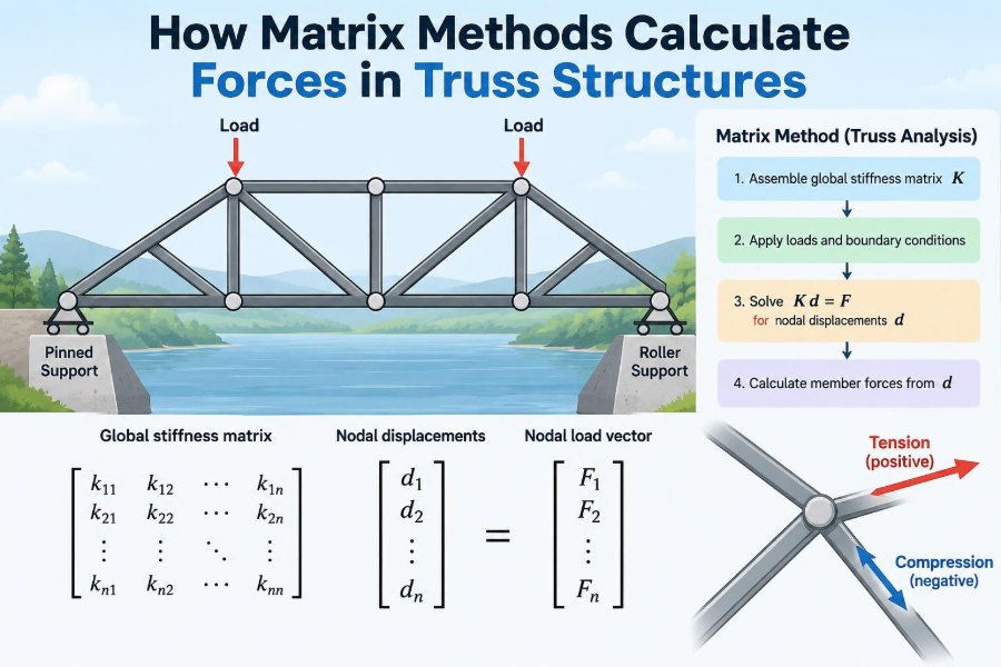
🌉 How Matrix Methods Calculate Forces in Truss Structures

A pedestrian bridge may look simple: straight steel members meeting at pinned joints, carrying people safely across a road or river. Yet every member must be sized for a force that changes with the load path, support arrangement, and geometry.

For a very small truss, an engineer can often calculate member forces with joint-by-joint equilibrium equations. For a roof truss, transmission tower, bridge span, or space-frame-like assembly, that approach soon becomes difficult to organise and easy to misapply.

Matrix methods turn many connected equilibrium and deformation relationships into one structured calculation. They are the foundation of the direct stiffness method and of much structural-analysis software used in engineering practice.

This article develops the logic behind the matrices rather than treating them as a black box. The goal is to see how nodal displacements lead to member extensions, member forces, reactions, and ultimately design decisions. 🏗️

🧭 1. What a truss model represents

A truss is an idealised structure made from straight, slender members connected at joints called nodes. In the classical model, loads and support reactions act only at nodes.

Each member carries only axial action: it is either in tension, being pulled, or compression, being pushed. It does not resist bending moment or shear in the idealisation.

Members are connected by frictionless pins.
Loads are applied at nodes.
Member centre lines meet at the nodes.
Each member has a known area, length, and elastic modulus.

Real joints and loads may depart from these assumptions, so model choice always matters as much as calculation. 🔍

🏗️ 2. Why matrices are useful for larger trusses

At every free joint in a two-dimensional truss, horizontal and vertical force equilibrium must be satisfied. A structure with many joints therefore produces a large, coupled collection of equations.

A matrix records this system compactly. It also provides a repeatable workflow: define nodes, assemble member contributions, impose supports, solve for displacements, then recover forces.

This organisation has practical advantages:

Repeated member calculations can be automated.
Geometry changes can be handled systematically.
Multiple load cases use the same structural matrix when properties stay linear.
Computer results can be checked against a transparent mathematical model.

📐 3. The central equation: KU = F

The key equation of linear structural analysis is K U = F. Here, K is the global stiffness matrix, U is the vector of nodal displacements, and F is the vector of applied nodal forces.

Stiffness means resistance to displacement. A large stiffness value means that a greater force is needed to produce a given displacement in a particular direction.

The equation is not merely a computational shortcut. It expresses equilibrium after every member’s force has been related to its deformation through material and geometric properties.

🧱 4. Start with nodes, members, and connectivity

Before forming a matrix, define a model unambiguously. Give every node a number and record its coordinates, then identify the two end nodes of every member.

This record is often called connectivity. For member e, connectivity might be written as (i, j), meaning that it joins node i to node j.

For each member, retain its cross-sectional area A and Young’s modulus E. If the structure uses different materials or member sizes, these properties can vary member by member.

🗺️ 5. Establish a global coordinate system

A planar truss is usually described using one global horizontal axis x and one global vertical axis y. Every nodal coordinate, load, displacement, and reaction is expressed in this common system.

Using global coordinates is essential because members point in different directions while joints must satisfy equilibrium in the same directions. A diagonal member cannot be assembled correctly until its local axial action is connected to global x and y components.

Choose a consistent positive direction at the start and keep it throughout the calculation.

🔢 6. Count degrees of freedom

A degree of freedom, or DOF, is an independent displacement component. Each node in a two-dimensional pin-jointed truss has two translational DOFs: one horizontal and one vertical.

For node i, a common ordering is uᵢ for horizontal displacement and vᵢ for vertical displacement. A truss with n nodes therefore starts with 2n global displacement entries.

Unlike a frame model, a pure truss node has no rotational DOF. Pin joints do not transfer member bending moments in the ideal truss formulation.

🧾 7. Build the displacement vector

The global displacement vector places all nodal translations in a declared order. For three nodes, one possible vector is:

U = [u₁  v₁  u₂  v₂  u₃  v₃]ᵀ

The superscript ᵀ means transpose, converting a row arrangement into a column vector. The exact numbering is not important, but consistency is.

Later, supports will prescribe some entries as zero or as a known settlement. The remaining entries are the unknown displacements solved by the matrix equation.

📏 8. Calculate a member’s geometry

For a member joining nodes i and j, first calculate coordinate differences:

Δx = xⱼ - xᵢ
Δy = yⱼ - yᵢ
L = √(Δx² + Δy²)

The quantity L is the member length. Its orientation is represented by the direction cosines c = Δx/L and s = Δy/L.

These values describe how strongly the member’s axial stiffness contributes to horizontal, vertical, and coupled global motion.

🧲 9. Recognise axial stiffness EA/L

A uniform bar under axial load follows the linear relation N = (EA/L) δ. In this expression, N is axial force and δ is axial extension, with signs determined by the chosen convention.

The factor EA/L is the member’s axial stiffness. A larger area or modulus increases stiffness, while a longer member decreases it.

This relationship comes from elastic strain: extension is proportional to force, length, and inverse material-area stiffness. It is the physical source of every truss stiffness matrix entry.

↔️ 10. See the local two-node bar

In a local coordinate system aligned with the member, only axial displacement matters. If u′₁ and u′₂ are the end displacements along the member axis, its local stiffness relation is:

[f′₁  f′₂]ᵀ = (EA/L) [ 1  -1
                        -1   1 ] [u′₁  u′₂]ᵀ

The opposite signs are important. Pulling one end relative to the other produces equal and opposite end forces, which respects Newton’s third law.

A member has no local stiffness against transverse motion in the ideal truss model.

🧩 11. Transform local action into global directions

Global nodal movement must be projected onto the member axis. For a member at angle θ, its direction cosines are c = cos θ and s = sin θ.

The axial extension caused by the global displacement vector is:

δ = [-c  -s  c  s] [uᵢ  vᵢ  uⱼ  vⱼ]ᵀ

This expression says that only the relative displacement component parallel to the member changes its length. A rigid translation of both ends produces no extension and no member force.

🧮 12. Form the 2D element stiffness matrix

After transformation to global axes, a two-dimensional truss member has a 4 × 4 element stiffness matrix:

kᵉ = (EA/L) [ c²   cs  -c²  -cs
               cs   s²  -cs  -s²
              -c² -cs   c²   cs
              -cs -s²   cs   s² ]

The associated DOFs are ordered as [uᵢ, vᵢ, uⱼ, vⱼ]. Terms such as cs show that a diagonal member couples horizontal and vertical motion.

A horizontal member has s = 0, so it contributes only horizontal stiffness. A vertical member has c = 0, so it contributes only vertical stiffness.

🧠 13. Interpret the matrix instead of memorising it

The element matrix is easier to trust when its structure is understood. The diagonal terms describe force at a DOF caused by movement at that same DOF, while off-diagonal terms describe coupling between connected DOFs.

Its rows sum to zero in the appropriate rigid-body sense. If both member ends move together without changing length, the member should create no internal axial force.

The matrix is also symmetric for a linear elastic bar: kᵉ = (kᵉ)ᵀ. This symmetry reflects reciprocal elastic behaviour and is a valuable checking clue.

🧷 14. Map element DOFs to global DOFs

Each member matrix only refers to four locations, but the global system contains all nodal DOFs. An assembly map identifies where the member’s four entries belong.

For a member joining nodes 2 and 5, using the ordering [u₁, v₁, u₂, v₂, ...], its map is:

[u₂, v₂, u₅, v₅] → [3, 4, 9, 10]

In software, this map is often generated directly from node numbers. On paper, writing it explicitly prevents a common and serious indexing error.

🧱 15. Assemble the global stiffness matrix

Assembly means adding each member’s 4 × 4 stiffness contributions into the corresponding rows and columns of the initially zero global matrix K.

Where multiple members meet at a joint, their contributions accumulate. That is physically correct: all connected members resist a nodal movement together.

The basic algorithm is simple:

Calculate kᵉ for one member.
Find its four global DOF indices.
Add every local entry to the matching global entry.
Repeat for every member.

🕸️ 16. Notice sparsity in real structural matrices

Most nodes connect to only a few nearby members. Therefore, most pairs of distant DOFs have no direct stiffness relationship, and many entries in a large global matrix are zero.

Such a matrix is called sparse. Efficient analysis programs exploit sparsity to reduce memory use and computational effort.

For learning calculations, a full matrix display is useful. For large structures, sparse storage and specialised solvers are far more practical.

📥 17. Create the global load vector

The vector F lists externally applied nodal forces in the same DOF order as U. A downward load has a negative vertical component if upward y is positive.

For example, a force at node 3 might contribute entries to positions for u₃ and v₃. A purely vertical applied load has zero horizontal component.

Distributed loads acting along a truss member require care. A classical truss model expects joint loads, so the loading idealisation must be justified before simply inserting force-vector values.

🛑 18. Model supports as displacement constraints

Supports are represented by known displacements, usually zero. A pin support in a planar truss restrains both horizontal and vertical translation, while a roller support commonly restrains one translation only.

The support description must match physical reality. Over-restraining a model can introduce artificial forces; under-restraining it can leave a mechanism that cannot resist load.

Idealised support	Typical restrained planar DOFs	Typical reaction components
Pin	`u = 0, v = 0`	Horizontal and vertical
Horizontal-surface roller	`v = 0`	Vertical
Fixed prescribed node	Specified translations	Components needed to enforce them

✂️ 19. Partition free and restrained DOFs

After identifying support constraints, rearrange the equations into free and restrained sets. In block form:

[Kff Kfr][Uf] = [Ff]
[Krf Krr][Ur]   [Fr]

Here Uf is unknown free displacement, while Ur is known restrained displacement. For ordinary fixed supports, Ur = 0.

The equation used to solve free movement is Kff Uf = Ff - Kfr Ur. This cleanly handles both zero restraints and prescribed support settlements.

🔓 20. Solve for nodal displacements

Once constraints are applied, solve the reduced linear system for Uf. These values are generally small translations, but their units must remain consistent with the chosen length units.

In numerical work, engineers typically use matrix factorisation methods rather than calculating an inverse explicitly. Writing Uf = Kff⁻¹Ff is useful algebraically, but direct inversion is usually not the preferred computational route.

The resulting deformed shape is often the most informative first output. It can expose an unexpected sway direction, a missing restraint, or a geometry error. 📉

📤 21. Recover support reactions

Reactions are not guessed from the supports; they follow from equilibrium after displacement is known. Using the full system, compute:

R = K U - F

At free DOFs, the residual should be approximately zero apart from numerical round-off. At restrained DOFs, the residual represents the support reaction required to enforce the specified displacement.

As an independent check, the total horizontal force, total vertical force, and total moment of all external loads and reactions should satisfy global equilibrium.

🧵 22. Recover extension and axial force in each member

Extract the four global displacement entries belonging to a member. Its axial extension is found by projection:

δ = [-c  -s  c  s] ue

The axial force is then N = (EA/L)δ. With the usual convention, positive N indicates tension and negative N indicates compression.

Reporting force signs clearly is essential. A magnitude without a tension-or-compression label is not enough for checking a truss member.

🔄 23. Distinguish member force, stress, and strain

These related quantities answer different questions. Member force describes the total axial action, stress describes intensity over area, and strain describes relative deformation.

Axial force: N
Stress: σ = N/A
Strain: ε = δ/L
Elastic relation: σ = Eε in the linear range

A member can have the same force as another but a different stress because its area differs. Compression members also require stability checks, not just stress checks.

⚠️ 24. Check stability before trusting a solution

A stiffness matrix may be singular or nearly singular if the truss can move as a rigid body or deform as a mechanism. In that case, the model lacks adequate restraint or triangulation.

For a planar truss, supports must prevent the necessary rigid-body translations and rotation of the whole assembly. Internal geometry must also prevent mechanisms, such as a pin-jointed rectangle changing shape without diagonal bracing.

A solver warning about singularity is not merely a software problem. It is often a meaningful message about the physical model.

🧪 25. Use simple checks to validate results

Matrix calculations can be internally consistent while still representing the wrong structure. Use independent checks at several stages.

Confirm all member lengths and direction cosines from a sketch.
Check that K is symmetric for this linear truss model.
Verify units in EA/L, loads, and displacements.
Check global force and moment equilibrium using reactions.
Inspect whether tension and compression patterns are physically plausible.
Compare a small model with the method of joints or sections.

For a conservative vertical load, an unconstrained upward movement at the loaded joint deserves investigation. 🧪

🧰 26. Avoid common modelling mistakes

Many errors are not advanced mathematics errors. They arise from a mismatch between the model and the intended structure.

Mixing millimetres with metres without converting stiffness consistently.
Swapping the end-node order in geometry but not in the displacement map.
Using an incorrect sign for a load or reaction.
Applying member loads as though the element were a beam.
Omitting a member property or assigning it to the wrong member.
Adding a rotational DOF to a truss formulation without an appropriate element model.

A labelled geometry sketch, a DOF table, and a sign convention written before calculation eliminate many of these failures.

💻 27. Understand what structural software is doing

Software can assemble thousands of elements quickly, but its core loop follows the same reasoning: calculate element matrices, assemble global stiffness, apply boundary conditions, solve displacements, and recover actions.

Understanding the workflow helps engineers review output intelligently. It becomes possible to question an unexpected reaction, identify an unstable release, or recognise when a result reflects an assumption rather than a physical fact.

Automation is most valuable when paired with engineering judgement. The computer solves the equations supplied; it cannot decide whether the idealisation is appropriate.

🌉 28. The core principle: compatibility, stiffness, and equilibrium

Matrix analysis works because three ideas are enforced at once. Compatibility makes connected members share nodal displacements, constitutive behaviour relates extension to axial force through EA/L, and equilibrium balances internal and external forces.

Each member contributes a small stiffness relation. Assembly combines those relations into one global model, supports supply displacement conditions, and the solution reveals how the whole truss moves and carries load.

When you understand that a truss force comes from member extension caused by compatible nodal displacement, the matrix method becomes a physical story—not just an array of numbers. 🌉 📐 ⚙️