📈 How Least-Squares Methods Find the Best-Fitting Model From Imperfect Data

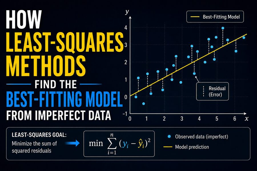
Real-world data is rarely perfect. Measurements contain noise, sensors have limited precision, experiments are affected by uncontrolled variables, and human observations introduce uncertainty. Yet scientists, engineers, economists, and data analysts still need to extract useful relationships from messy information. 📊

One of the most important mathematical tools for doing this is the least-squares method.

Least squares finds a model that comes as close as possible to a collection of observed data points by minimizing the total squared difference between the model’s predictions and the actual measurements.

It is used in linear regression, curve fitting, calibration, signal processing, machine learning, navigation, astronomy, finance, and countless other fields.

The core idea is surprisingly simple:

Choose the model whose predictions produce the smallest total squared error. 🎯

Behind that straightforward principle lies a powerful framework that helps transform imperfect observations into useful mathematical models.

📍 1. Why Data Rarely Fits a Perfect Equation

Suppose an engineer measures how far a spring stretches under different loads.

If the spring behaved perfectly and every measurement were exact, all data points might lie precisely on a straight line.

In reality, the measurements could look something like:

Load	Measured Extension
1	2.1
2	3.9
3	6.2
4	7.8
5	10.1

The points appear approximately linear, but they do not fall exactly on one line.

Why?

Possible causes include:

• Measurement noise
• Instrument calibration errors
• Temperature changes
• Material imperfections
• Human reading errors
• Unmodeled physical effects

Instead of demanding a line that passes through every point, we look for the line that represents the overall trend as well as possible.

That is the problem least squares solves. 📐

📏 2. Start With a Mathematical Model

For a simple straight-line relationship, the model is:

y = mx + b

where:

• x is the input
• y is the predicted output
• m is the slope
• b is the intercept

The challenge is to determine the values of m and b that best match the observed data.

Different choices produce different lines.

One line may pass close to the first few points but miss the later ones.

Another may fit the middle well while performing poorly at the edges.

Least squares gives us an objective rule for deciding which line is best.

🎯 3. What Is a Residual?

For every data point, the model makes a prediction.

Suppose an observation has actual value:

yᵢ

and the model predicts:

ŷᵢ

The difference is called the residual:

rᵢ = yᵢ − ŷᵢ

If the residual is positive, the actual data point lies above the model.

If it is negative, the point lies below the model.

A perfect prediction would have a residual of zero.

Least squares tries to make these residuals collectively as small as possible. 📉

➕ 4. Why Not Simply Add the Errors?

At first, we might try to add all residuals:

r₁ + r₂ + r₃ + …

Unfortunately, this does not work well.

Positive and negative residuals can cancel each other.

For example:

+5 + (-5) = 0

A total residual of zero could therefore occur even when the model is badly wrong.

We need a way to measure error without allowing cancellation.

One possibility would be taking absolute values.

Least squares instead uses squared residuals.

🔢 5. The Least-Squares Objective

Each residual is squared:

rᵢ² = (yᵢ − ŷᵢ)²

Then all squared residuals are added:

S = Σ(yᵢ − ŷᵢ)²

This quantity is called the sum of squared errors, residual sum of squares, or sum of squared residuals, depending on context.

Least squares chooses the model parameters that make S as small as possible.

For a straight line:

S(m,b) = Σ[yᵢ − (mxᵢ + b)]²

The best-fitting values of m and b are the ones that minimize this expression. 🧮

🟦 6. Why Square the Errors?

Squaring residuals provides several useful properties.

First, all squared values are nonnegative.

A residual of -4 and a residual of +4 both contribute:

16

So cancellation disappears.

Second, large errors receive stronger penalties.

For example:

• Error of 1 → squared error = 1
• Error of 2 → squared error = 4
• Error of 5 → squared error = 25
• Error of 10 → squared error = 100

Large deviations therefore influence the fitted model much more strongly than small ones.

Third, squared-error functions are smooth and mathematically convenient to differentiate.

This makes optimization much easier.

📐 7. Finding the Best-Fitting Straight Line

For ordinary linear least squares, the goal is to minimize:

Σ[yᵢ − (mxᵢ + b)]²

Because this expression is differentiable, calculus can be used.

We take partial derivatives with respect to m and b, set them equal to zero, and solve the resulting equations.

These are known as the normal equations.

For simple linear regression, the slope can be calculated as:

m = Σ(xᵢ − x̄)(yᵢ − ȳ) / Σ(xᵢ − x̄)²

The intercept is then:

b = ȳ − mx̄

where x̄ and ȳ are the average values of x and y.

This gives the unique least-squares line when the inputs contain sufficient variation.

📊 8. A Simple Example

Suppose we have three observations:

(1, 2)
(2, 3)
(3, 5)

These points are not perfectly collinear.

A least-squares calculation produces a line close to:

y = 1.5x + 0.33

The predictions are approximately:

• x = 1 → 1.83
• x = 2 → 3.33
• x = 3 → 4.83

The residuals are therefore small.

The line does not pass through every observation, but it balances the errors across all of them.

That is the key idea: the model is not trying to explain every measurement perfectly. It is finding the best overall compromise. ⚖️

🧠 9. Least Squares Is an Optimization Problem

Least-squares fitting can be viewed as an optimization task.

We have:

Parameters: values we can change
Objective function: total squared error
Goal: minimize that function

This idea extends far beyond straight lines.

A model might contain dozens, thousands, or even millions of adjustable parameters.

The principle remains the same:

1. Make predictions.
2. Compare predictions with observations.
3. Square the errors.
4. Add them together.
5. Adjust parameters to reduce the total.

Modern machine learning uses closely related optimization ideas on enormous datasets. 🤖

📈 10. Least Squares Can Fit More Than Straight Lines

Despite being strongly associated with linear regression, least squares is not limited to fitting straight lines.

Suppose we want to fit a quadratic:

y = ax² + bx + c

We can choose a, b, and c to minimize the squared residuals.

Similarly, least squares can fit:

• Polynomial curves
• Sinusoidal models
• Exponential relationships
• Multiple-variable regression models
• Physical system models
• Calibration functions

The important requirement is not necessarily that the curve itself be visually straight.

What matters is how the unknown parameters enter the optimization problem.

🧮 11. Multiple Linear Regression

Real-world predictions often depend on several variables.

For example, suppose a model predicts house price from:

• Floor area
• Number of bedrooms
• Age
• Distance from city center

A linear model might look like:

Price = β₀ + β₁Area + β₂Bedrooms + β₃Age + β₄Distance

The coefficients β₀, β₁, ... are selected using least squares.

Instead of fitting a line in two dimensions, the method is fitting a plane or hyperplane in a higher-dimensional space.

The mathematics generalizes naturally using matrices.

🧱 12. The Matrix Form of Least Squares

A linear least-squares problem is often written compactly as:

Ax ≈ b

Here:

• A contains known input data
• x contains unknown model parameters
• b contains observed outputs

Because the observations are imperfect, there may be no exact x satisfying:

Ax = b

Least squares therefore finds the x minimizing:

||Ax − b||²

The classical normal-equation solution is:

AᵀAx = Aᵀb

and, when the relevant inverse exists:

x = (AᵀA)⁻¹Aᵀb

This formula is mathematically elegant, although numerical software often uses better computational methods than explicitly forming the inverse.

💻 13. Why Computers Often Use QR Decomposition

Directly calculating (AᵀA)⁻¹ can be numerically unstable, especially when columns of A are nearly dependent or the data span very different scales.

Practical numerical software therefore often solves least-squares problems using methods such as:

• QR decomposition
• Singular Value Decomposition (SVD)

QR decomposition expresses a matrix approximately as:

A = QR

where Q has orthogonal columns and R is triangular.

This transforms the fitting problem into one that is usually more stable to solve.

For challenging or rank-deficient problems, SVD can be even more robust. 🖥️

📐 14. The Geometric Meaning of Least Squares

Least squares also has a beautiful geometric interpretation.

Imagine the observed data vector b lying outside the space of vectors that the model can produce.

The model cannot reproduce b exactly.

Instead, least squares finds the model output Ax that lies closest to b.

Geometrically, the residual:

b − Ax

is perpendicular to the model’s column space at the optimum.

This is why the normal equations contain:

Aᵀ(b − Ax) = 0

The residual is orthogonal to every direction available to the model.

Least squares is therefore essentially a projection problem. 📐

🎲 15. Why Least Squares Has a Statistical Interpretation

Least squares is not merely a geometric trick.

It also has an important statistical justification.

Suppose measurement errors are:

• Independent
• Centered around zero
• Normally distributed
• Of equal variance

Under these assumptions, the least-squares solution is also the maximum likelihood estimate of the model parameters.

In other words, the least-squares model is the one that makes the observed data most statistically plausible under Gaussian noise.

This connection helps explain why least squares appears so often in statistics and scientific measurement.

⚠️ 16. Outliers Can Strongly Affect the Result

Squaring residuals has an important downside.

Large errors receive very large penalties.

Suppose most residuals are around 1 or 2, but one unusual point has an error of 20.

Its squared error is:

400

That single point can heavily influence the entire fitted model.

Such unusual observations are called outliers.

Outliers may result from:

• Sensor failure
• Data-entry mistakes
• Rare events
• Incorrect assumptions
• Genuine extreme observations

Because least squares is sensitive to them, analysts should inspect data carefully rather than blindly trusting a fitted line. 🔍

🛡️ 17. Robust Regression Handles Outliers Differently

When outliers are common, alternatives to ordinary least squares may perform better.

One option is least absolute deviations, which minimizes:

Σ|yᵢ − ŷᵢ|

Another approach uses robust loss functions such as the Huber loss, which behaves like squared error for small deviations but penalizes very large errors less aggressively.

Robust methods can prevent a few extreme observations from dominating the model.

However, they may require more complicated optimization procedures.

⚖️ 18. Weighted Least Squares

Ordinary least squares treats every observation equally.

But sometimes certain measurements are more reliable than others.

Suppose one instrument measures with extremely high precision while another has much greater uncertainty.

It may be reasonable to give the precise observations more influence.

Weighted least squares minimizes:

Σwᵢ(yᵢ − ŷᵢ)²

where wᵢ is the weight assigned to each observation.

Higher weights make the corresponding residuals matter more.

Weighted least squares is common in experimental science where measurement uncertainties are known. 🔬

📏 19. Residuals Reveal Whether the Model Makes Sense

After fitting a model, analysts should examine the residuals.

If the model is appropriate, residuals may appear roughly random around zero.

But patterns can indicate problems.

For example:

• Curved residual pattern → relationship may not be linear
• Increasing residual spread → changing variance
• Repeating pattern → missing time dependence
• Clusters → missing categorical variables
• Large isolated residuals → possible outliers

Residual analysis therefore helps determine whether a model is merely mathematically fitted or actually appropriate for the data.

🎯 20. A Small Error Does Not Guarantee a Good Model

A least-squares algorithm will always try to find the best fit among the models it is allowed to use.

That does not mean the chosen model is scientifically correct.

Suppose we fit a straight line to data generated by a strong curved relationship.

Least squares will still find the best straight line.

But the line may be a poor description of the underlying process.

This distinction is essential:

Least squares finds the best model within a chosen model family—it does not prove that the model family itself is correct.

Good modeling requires domain knowledge as well as mathematics. 🧠

🔬 21. Applications in Science and Engineering

Least squares appears throughout scientific measurement.

Astronomers use fitting methods to estimate orbital parameters and analyze observations. 🌌

Engineers calibrate sensors by comparing known inputs with measured outputs.

Surveyors estimate locations from imperfect distance and angle measurements.

Signal-processing systems fit waveforms to noisy measurements.

Chemists estimate reaction parameters from experimental data.

Navigation systems combine uncertain observations to estimate position and motion.

In each case, there are more imperfect observations than can be satisfied exactly, so least squares helps find the most consistent model.

🤖 22. Least Squares in Machine Learning

Linear regression is one of the foundational algorithms in machine learning.

Given input features and known target values, least squares finds coefficients that minimize prediction error.

For example, a model might predict energy consumption using:

• Temperature
• Building size
• Time of day
• Occupancy

During training, the model adjusts its parameters to reduce squared error across the training data.

More complex neural networks often use variants of squared-error loss for certain tasks, although many applications use other loss functions better suited to classification or probabilistic outputs.

Least squares therefore represents one of the simplest examples of the broader machine-learning principle of minimizing a loss function. 🤖📊

🧪 23. Overfitting Is Still Possible

Suppose we have ten noisy data points.

A straight line may leave moderate residuals.

A very high-degree polynomial might pass through every single point exactly.

Its training error could become zero.

Does that make it better?

Not necessarily.

The complicated polynomial may simply memorize noise rather than capture the true underlying relationship.

This is called overfitting.

A good model should not only fit existing measurements; it should also make sensible predictions for new data.

Least squares therefore often works together with techniques such as:

• Cross-validation
• Regularization
• Model selection
• Validation datasets

🧲 24. Regularized Least Squares

Regularization adds a penalty for overly large or complicated model parameters.

For example, ridge regression minimizes:

Σ(yᵢ − ŷᵢ)² + λΣβⱼ²

The first term measures fitting error.

The second discourages excessively large coefficients.

The parameter λ controls the strength of regularization.

Regularization can improve stability, reduce overfitting, and help when predictor variables are strongly correlated.

This extends the least-squares idea from simply fitting observations toward finding models that balance accuracy and simplicity. ⚖️

📉 25. Measuring How Good the Fit Is

After fitting a model, several statistics can help evaluate performance.

One common quantity is the mean squared error, or MSE:

MSE = (1/n)Σ(yᵢ − ŷᵢ)²

Another is the root mean squared error, or RMSE:

RMSE = √MSE

RMSE is useful because it has the same units as the original output variable.

In regression analysis, another familiar measure is R², or the coefficient of determination.

R² summarizes how much of the observed variation is explained by the model, although it should not be treated as the only measure of model quality.

🌍 26. Why Least Squares Became So Important

Least squares dates back more than two centuries and is associated with mathematicians such as Adrien-Marie Legendre and Carl Friedrich Gauss.

Its enduring importance comes from a rare combination of properties:

• Conceptually simple
• Mathematically elegant
• Computationally efficient
• Statistically meaningful
• Easily generalized
• Useful across many scientific disciplines

Modern computers can solve least-squares problems involving enormous datasets, but the fundamental principle remains the same as in early astronomical calculations.

Find the parameters that make the squared discrepancies between prediction and observation as small as possible.

🧠 Conclusion

Least-squares methods provide a systematic way to turn imperfect data into useful mathematical models.

The process begins with a set of observations and a chosen model. For each observation, the model produces a prediction. The difference between prediction and reality is the residual.

Least squares then squares those residuals and adds them together:

Σ(yᵢ − ŷᵢ)²

The best-fitting parameters are those that minimize this total. 🎯

For simple linear regression, the solution can be derived directly with calculus. For larger problems, matrix methods such as QR decomposition and SVD provide efficient and numerically stable solutions.

The technique works because it balances errors across all observations rather than trying to force an exact fit to noisy data.

Yet least squares must be used thoughtfully. Outliers can distort results, inappropriate model assumptions can produce misleading conclusions, and excessive model complexity can lead to overfitting.

Despite these limitations, least squares remains one of the foundational tools of applied mathematics.

Whenever scientists estimate a trend from noisy measurements, engineers calibrate equipment, analysts build regression models, or computers infer relationships from imperfect data, the same elegant idea is often operating underneath:

Do not demand perfection from imperfect observations. Instead, find the model that makes the total disagreement as small as possible. 📈🧮✨