📐 How the Newton–Raphson Method Finds Solutions to Difficult Nonlinear Equations

Many equations can be solved with familiar algebra. If we have:

2x + 4 = 10

we can isolate x and quickly find:

x = 3

But not every equation is so cooperative. In science, engineering, economics, physics, machine learning, and numerical computing, we often encounter nonlinear equations whose solutions cannot be written down easily using ordinary algebraic formulas. 🧮⚙️

Examples include equations such as:

x³ − x − 2 = 0

cos(x) = x

e⁻ˣ = x

These equations may have one solution, several solutions, or sometimes no real solution at all.

When a clean symbolic answer is difficult or impossible to obtain, numerical methods become extremely important.

One of the most famous and powerful of these methods is the Newton–Raphson method, also commonly called Newton’s method.

Its central idea is beautifully simple:

Start with a guess, use the slope of the function to predict a better guess, and repeat until the answer stops changing significantly. 🔁📉

🧠 What Problem Does Newton–Raphson Solve?

Suppose we want to solve an equation of the form:

f(x) = 0

The goal is to find a value of x where the function crosses or touches the horizontal axis.

That value is called a root or zero of the function.

For example, consider:

f(x) = x² − 2

Solving:

x² − 2 = 0

means finding:

x = √2

The positive solution is approximately:

1.41421356…

Newton–Raphson can find this value numerically even if we begin with only a rough initial estimate.

📈 The Geometric Idea Behind Newton’s Method

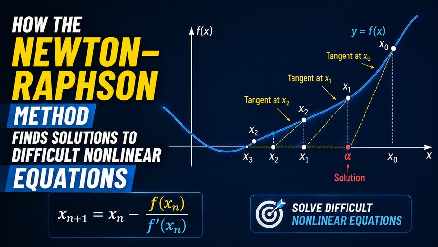
The Newton–Raphson method uses the tangent line to a curve.

Imagine graphing a nonlinear function f(x).

You choose an initial guess:

x₀

The point on the curve is:

(x₀, f(x₀))

At that point, draw a tangent line.

The tangent line has nearly the same direction as the curve locally.

Now extend that tangent line until it crosses the x-axis.

That intersection gives a new estimate:

x₁

Then repeat the process:

Evaluate the function at x₁.
Draw the tangent there.
Find where the tangent meets the x-axis.
Call that new point x₂.
Continue.

If the method behaves well, the sequence:

x₀, x₁, x₂, x₃, …

moves closer and closer to the actual root. 🎯

🧮 Deriving the Newton–Raphson Formula

The tangent line at a point xₙ has slope:

f′(xₙ)

Using the point-slope form of a line:

y − f(xₙ) = f′(xₙ)(x − xₙ)

We want to know where the tangent crosses the x-axis.

At that point:

y = 0

So:

0 − f(xₙ) = f′(xₙ)(xₙ₊₁ − xₙ)

Solving for the next estimate gives the famous formula:

xₙ₊₁ = xₙ − f(xₙ) / f′(xₙ)

This single expression is the heart of the Newton–Raphson method. ❤️🧮

It says:

Next guess = Current guess − Function value ÷ Slope

🔢 Example: Finding √2

Let us solve:

x² − 2 = 0

Define:

f(x) = x² − 2

Its derivative is:

f′(x) = 2x

The Newton formula becomes:

xₙ₊₁ = xₙ − (xₙ² − 2)/(2xₙ)

Suppose we begin with:

x₀ = 1.5

First iteration

Evaluate:

f(1.5) = 1.5² − 2 = 0.25

and:

f′(1.5) = 3

Then:

x₁ = 1.5 − 0.25/3

x₁ ≈ 1.4166667

Already, this is close to √2.

Second iteration

Using x₁ ≈ 1.4166667:

x₂ ≈ 1.4142157

Third iteration

One more step gives approximately:

x₃ ≈ 1.41421356

That is accurate to many decimal places.

Only a few iterations were needed. ⚡

🚀 Why Newton–Raphson Can Converge So Quickly

Newton’s method is famous for its speed near a well-behaved root.

Under suitable mathematical conditions, it exhibits quadratic convergence.

This roughly means that once the estimate is sufficiently close to the solution, the number of correct digits can approximately double with each iteration.

For example, the sequence might improve like this:

1 correct digit
2 correct digits
4 correct digits
8 correct digits

This makes Newton–Raphson extremely efficient compared with slower methods that only reduce the error by a fixed factor each step.

However, fast convergence is not guaranteed in every problem. ⚠️

🎯 The Importance of the Initial Guess

The starting value, called the initial guess, can strongly affect the method.

Suppose an equation has multiple roots.

Different starting guesses may lead to different solutions.

For example:

f(x) = x² − 4

has roots:

x = −2

and:

x = 2

A starting guess near +2 will usually converge to the positive root.

A starting guess near −2 will usually converge to the negative root.

So Newton’s method is not simply asking:

“What is the solution?”

It is often asking:

“Which solution is close to my starting point?” 📍

⚠️ What Happens If the Derivative Is Zero?

The Newton formula contains:

f′(xₙ)

in the denominator.

If:

f′(xₙ) = 0

then the method attempts to divide by zero.

This means the tangent line is horizontal and does not give a useful x-axis intersection.

Even if the derivative is merely very small, the correction:

f(xₙ) / f′(xₙ)

can become extremely large.

The next estimate may jump far away from the root. 🚨

This is one of the method’s most important limitations.

🔄 Newton’s Method Can Sometimes Oscillate

Newton–Raphson does not always move steadily toward a root.

In some cases, the estimates can bounce back and forth.

For example:

x₀ → x₁ → x₂ → x₁ → x₂ → …

The method can become trapped in a cycle.

This may happen when the function has certain shapes or when the initial guess is poorly chosen.

Numerical software often protects against this by:

Limiting step size
Using a maximum number of iterations
Combining Newton’s method with safer methods
Testing whether the residual is actually decreasing

💥 Newton’s Method Can Diverge

In some problems, Newton iterations move farther and farther from the solution.

This behavior is called divergence.

Suppose the tangent line at the current point crosses the x-axis far away from any useful root.

The next guess may be worse than the previous one.

Repeated poor steps can send the estimate toward very large values or into unstable regions.

Therefore, Newton–Raphson is powerful but not foolproof.

Good numerical algorithms monitor convergence rather than blindly assuming every iteration improves the answer.

📉 What Does “Convergence” Mean?

A numerical method is said to converge when its sequence of approximations approaches a solution.

In practice, computers must decide when to stop.

One common criterion is:

|xₙ₊₁ − xₙ| < tolerance

For example:

tolerance = 0.000001

Another useful test is checking the residual:

|f(xₙ)| < tolerance

A robust implementation often checks both.

This is important because two successive guesses could be similar even if they are not actually near a true root.

🧪 Example: Solving cos(x) = x

Consider:

cos(x) = x

Rewrite it as:

f(x) = cos(x) − x

Then:

f′(x) = −sin(x) − 1

Newton’s formula becomes:

xₙ₊₁ = xₙ − [cos(xₙ) − xₙ]/[−sin(xₙ) − 1]

Starting with:

x₀ = 1

the sequence rapidly approaches:

x ≈ 0.739085…

This number has no simple elementary closed-form expression, yet Newton–Raphson finds it efficiently.

That illustrates one of the method’s biggest strengths: solving equations that resist ordinary algebra. 🔍

🛠️ Newton–Raphson in Engineering

Engineers frequently encounter nonlinear equations.

Examples include:

Electrical circuits ⚡
Fluid flow 💧
Structural mechanics 🏗️
Chemical equilibrium 🧪
Heat transfer 🌡️
Control systems 🎛️
Power-system analysis 🔌

For instance, electrical networks often contain nonlinear components.

A diode’s current-voltage relationship is exponential rather than linear.

To determine the operating point of a circuit containing diodes or transistors, circuit simulators may repeatedly solve nonlinear equations using Newton-like methods.

Without such numerical techniques, tools such as SPICE would be far less useful.

⚡ Newton–Raphson in Power-Flow Analysis

Electrical power grids provide another major application.

Engineers need to determine:

Voltage magnitudes
Voltage angles
Active power
Reactive power

at many buses in a power network.

The governing power-flow equations are nonlinear.

Newton–Raphson methods are widely used because they can solve large coupled systems efficiently.

Instead of a single unknown x, engineers may need to solve hundreds or thousands of variables simultaneously.

The basic idea remains similar, but derivatives become matrices. 📊

🧩 Extending Newton’s Method to Multiple Variables

Suppose we have several nonlinear equations:

f₁(x, y) = 0

f₂(x, y) = 0

Now the unknown is not a single number but a vector.

Instead of an ordinary derivative, we use a matrix of partial derivatives called the Jacobian matrix.

For a system:

F(x) = 0

the multidimensional Newton step is commonly written conceptually as:

J(xₙ) Δx = −F(xₙ)

Then:

xₙ₊₁ = xₙ + Δx

where J is the Jacobian.

Rather than explicitly calculating a matrix inverse, numerical software usually solves the associated linear system directly.

This extension makes Newton’s method one of the foundational tools of scientific computing. 💻

📐 What Is the Jacobian Matrix?

For two functions:

f₁(x, y)

and

f₂(x, y)

the Jacobian is:

[ ∂f₁/∂x   ∂f₁/∂y ]
[ ∂f₂/∂x   ∂f₂/∂y ]

Each entry describes how one equation changes when one variable changes.

The Jacobian plays a role similar to the derivative in the one-dimensional method.

It tells the algorithm how the nonlinear system behaves locally.

Using this local linear approximation, Newton’s method predicts how the variables should change to move closer to a solution.

🔍 Newton’s Method Is Really Local Linearization

One of the deepest ways to understand Newton–Raphson is as a linear approximation method.

Nonlinear functions are difficult because they bend and curve.

But over a small region, a smooth nonlinear function can often be approximated by a straight line.

Newton’s method repeatedly does this:

Replace the nonlinear function locally with a tangent line.
Solve the simple linear approximation.
Move to the new point.
Rebuild the approximation.
Repeat.

So Newton’s method transforms a difficult nonlinear problem into a sequence of easier linear problems. 🧠✨

🆚 Newton–Raphson vs Bisection

Another popular root-finding method is the bisection method.

Bisection starts with an interval:

[a, b]

where the function changes sign.

It repeatedly cuts the interval in half.

Advantages of Bisection

Very reliable
Simple to implement
Does not require derivatives
Guaranteed to converge under standard conditions

Disadvantages

Usually slower than Newton’s method
Requires a valid bracketing interval

Newton–Raphson is almost the opposite.

Advantages of Newton–Raphson

Very fast near a root
Often needs only a few iterations
Excellent for large scientific problems

Disadvantages

Requires derivative information
Can diverge
Sensitive to initial guesses
May fail near zero derivatives

For this reason, many robust numerical solvers combine both strategies. ⚖️

🔄 Newton–Raphson vs Secant Method

The secant method is similar to Newton’s method but avoids explicitly computing a derivative.

Instead, it estimates the slope using two previous points.

Conceptually:

Derivative ≈ change in function / change in x

This can be useful when derivatives are expensive or unavailable.

The secant method is often faster than bisection but generally does not achieve the same local quadratic convergence as standard Newton–Raphson.

It represents a compromise between derivative-free simplicity and Newton-style speed.

🧠 How Are Derivatives Obtained in Real Software?

For simple equations, derivatives can be calculated by hand.

Large scientific programs have several options.

✍️ Analytical Differentiation

A mathematician or engineer derives the derivative formula explicitly.

This can be very accurate but labor-intensive.

🔢 Numerical Differentiation

The derivative is approximated using nearby function values.

For example:

f′(x) ≈ [f(x + h) − f(x)] / h

This is convenient but introduces approximation error.

🤖 Automatic Differentiation

Modern software can compute derivatives automatically by applying differentiation rules to computer operations.

Automatic differentiation is especially important in:

Machine learning
Optimization
Scientific computing
Simulation software

It provides highly accurate derivatives without requiring manual symbolic derivation.

🤖 Newton’s Method and Optimization

Newton’s method is also closely related to optimization.

Suppose we want to minimize a function:

g(x)

At a minimum, under appropriate smoothness conditions:

g′(x) = 0

So finding a minimum becomes a root-finding problem for the derivative.

Apply Newton’s method to:

f(x) = g′(x)

Then:

f′(x) = g″(x)

The update becomes:

xₙ₊₁ = xₙ − g′(xₙ)/g″(xₙ)

This is known as Newton’s optimization method.

In multiple dimensions, the second-derivative matrix is called the Hessian.

Newton-style optimization is used in statistics, machine learning, economics, and many other fields. 📊🤖

📉 Why Newton’s Method Can Beat Gradient Descent

Gradient descent moves according to the slope.

Newton’s optimization method uses both:

First derivatives
Second derivatives

The second derivative provides information about curvature.

Imagine descending into a valley.

Gradient descent knows which direction is downhill.

Newton’s method also estimates how sharply the landscape curves.

That additional information can allow much larger and more intelligent steps.

However, calculating and solving systems involving the Hessian can be expensive for very large problems.

This motivates methods such as:

Quasi-Newton methods
BFGS
L-BFGS

These attempt to capture some of Newton’s speed without explicitly computing the full second-derivative matrix.

🧪 Repeated Roots Can Slow Convergence

Newton–Raphson’s famous quadratic speed does not always apply.

Suppose a function has a repeated root, such as:

f(x) = (x − 2)²

The root is:

x = 2

But the function only touches the x-axis instead of crossing it.

Standard Newton iterations may converge more slowly in this situation.

If the multiplicity of the root is known, modified Newton formulas can restore faster convergence.

This demonstrates that the geometry of the function strongly influences numerical behavior.

🚧 Why Numerical Safeguards Matter

Professional numerical libraries rarely implement the simplest textbook Newton formula without protection.

A robust solver may include:

Maximum iteration counts
Derivative magnitude checks
Step-size limits
Line searches
Trust regions
Bracketing intervals
Residual monitoring
NaN and overflow detection

These safeguards make the algorithm far more reliable in real applications.

The goal is not merely to make progress quickly but to avoid catastrophic steps when the local tangent approximation is poor. 🛡️

🎯 Damped Newton Methods

Sometimes the full Newton step is too aggressive.

Instead of using:

xₙ₊₁ = xₙ + Δx

a damped method may use:

xₙ₊₁ = xₙ + αΔx

where:

0 < α ≤ 1

If α = 1, we take the full Newton step.

If α = 0.5, we move only halfway.

Reducing the step size can help prevent divergence and improve stability.

Optimization algorithms often choose α using a line search.

🧭 Trust-Region Methods

Another strategy is the trust-region approach.

Instead of trusting the local linear or quadratic approximation everywhere, the algorithm limits the step to a region where the approximation is believed to be reliable.

If the predicted improvement matches reality, the trust region can expand.

If the prediction is poor, the region shrinks.

Trust-region methods are widely used in advanced nonlinear optimization because they combine Newton-like efficiency with greater robustness.

💻 A Simple Newton–Raphson Algorithm

Conceptually, the algorithm looks like this:

Choose initial guess x

Repeat:
    fx  = f(x)
    dfx = f'(x)

    if derivative is too small:
        stop or use another method

    new_x = x - fx / dfx

    if |new_x - x| is sufficiently small:
        return new_x

    x = new_x

Real implementations also check the residual and enforce iteration limits.

Despite its enormous importance, the basic algorithm is surprisingly compact. 💡

🌍 Where Newton–Raphson Is Used

Newton’s method and its variants appear across countless disciplines:

⚡ Circuit simulation
🔌 Electrical power-flow calculations
🧪 Chemical process modeling
🛰️ Orbital mechanics
🌡️ Heat-transfer calculations
🚀 Aerospace engineering
💧 Fluid dynamics
🏗️ Structural analysis
📈 Economics
💹 Financial modeling
🤖 Machine learning
📊 Statistical estimation
🎮 Physics engines
🔬 Scientific simulation

Whenever nonlinear equations appear, Newton-style algorithms are likely nearby.

🛰️ Example in Orbital Mechanics

Orbital calculations often require solving Kepler’s equation:

M = E − e sin(E)

where:

M is mean anomaly
E is eccentric anomaly
e is orbital eccentricity

The variable E appears both directly and inside a sine function.

There is no general elementary algebraic rearrangement that isolates E.

Newton–Raphson can solve it efficiently.

Satellite-navigation and astronomy calculations frequently rely on numerical methods of this kind. 🛰️🌌

🧪 Example in Chemical Engineering

Chemical equilibrium calculations often involve nonlinear relationships between:

Temperature
Pressure
Composition
Equilibrium constants

Multiple nonlinear equations may need to be satisfied simultaneously.

Newton-based solvers can repeatedly linearize the equations and update the estimated chemical composition.

This makes them critical in process simulators used to design reactors, distillation systems, and other industrial equipment.

🧠 Why Newton’s Method Is So Important

Newton–Raphson is not valuable simply because it solves one particular equation.

Its importance comes from a much broader principle:

Use local derivative information to transform a nonlinear problem into a sequence of manageable approximations.

That idea appears throughout numerical mathematics.

Once the method is generalized to systems, optimization, and large sparse matrices, it becomes one of the foundational frameworks behind modern simulation and computational engineering.

⚠️ When Newton–Raphson Is a Poor Choice

Newton’s method may not be ideal when:

The derivative is unavailable
Derivatives are extremely expensive
The starting guess is poor
The function is discontinuous
The function has sharp corners
The derivative becomes zero
Global convergence is more important than speed
Many roots must be found systematically

In such cases, other methods such as bisection, secant, Brent’s method, or specialized nonlinear solvers may be preferable.

There is no universally best root-finding algorithm.

🔮 Modern Improvements to Newton’s Method

Contemporary numerical software has developed many variations of Newton’s original idea.

Examples include:

Damped Newton methods
Inexact Newton methods
Newton–Krylov methods
Quasi-Newton algorithms
Trust-region Newton methods
Sparse Newton solvers

These variants address problems involving millions of variables, expensive derivatives, noisy data, or poorly conditioned systems.

The basic tangent-line concept has therefore evolved into a massive family of computational techniques. 🚀

📌 A Useful Mental Picture

The easiest way to remember Newton–Raphson is to imagine standing somewhere on a curved hill.

You look at the slope directly beneath your feet.

Then you pretend that the local slope continues as a straight line.

Where would that straight line reach ground level?

Move there.

Then measure the new slope and repeat.

Each tangent is only a local approximation, but when the function is smooth and the starting point is good, those approximations rapidly guide you toward the root. 📉🎯

🏁 Final Thoughts

The Newton–Raphson method solves difficult nonlinear equations by repeatedly replacing a curved function with a simple tangent-line approximation.

Beginning with an initial estimate xₙ, it computes:

xₙ₊₁ = xₙ − f(xₙ)/f′(xₙ)

The function value tells the algorithm how far the current point is from satisfying the equation, while the derivative indicates the local direction and steepness of the curve.

Together, those two pieces of information produce a new estimate that can be dramatically better than the previous one.

When conditions are favorable, Newton’s method converges extraordinarily quickly—often producing many accurate digits after only a handful of iterations. ⚡

Its power comes with limitations. Poor initial guesses, small derivatives, multiple roots, or difficult function geometry can cause slow convergence, oscillation, or complete divergence.

That is why real numerical software often combines Newton’s method with damping, line searches, trust regions, or safer root-bracketing techniques.

Even so, the central idea remains one of the most elegant in numerical mathematics:

Approximate the nonlinear problem locally, solve the simpler approximation, and repeat until the approximation becomes the solution. 🧮✨

From finding square roots in simple demonstrations to solving enormous systems in power grids, chemical plants, satellite calculations, machine learning, and engineering simulations, Newton–Raphson remains one of the most influential algorithms ever developed for numerical problem solving. 🌍📐🚀