
A bridge deck begins to vibrate after a gust of wind. A motor shaft develops an unexpected hum. A power network experiences a small disturbance that either fades away or grows into a serious instability.
Engineers need more than a list of measurements to understand these situations. They need to identify the system’s natural patterns of behaviour, determine which patterns dominate, and predict whether they are safe.
Eigenvalues and eigenvectors provide that information. They turn a coupled engineering system into meaningful modes: characteristic shapes, directions, frequencies, growth rates, or principal stresses.
Although the mathematics begins with matrices, the engineering interpretation is practical. It helps designers diagnose vibration, control machines, analyse structures, process signals, and model changing systems. ⚙️
🧭 1. The central engineering question
Many engineering models relate an input or state vector to another vector through a matrix. The matrix may represent stiffness, inertia, heat transfer, electrical coupling, or a linearized dynamic system.
The key question is: which directions or patterns are preserved by this transformation? Those special patterns are eigenvectors, and the associated scaling factors are eigenvalues.
📐 2. The defining equation
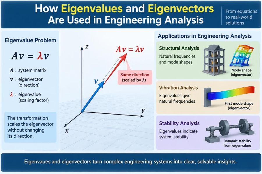
For a square matrix A, an eigenvector v and eigenvalue λ satisfy:
Av = λv
The vector changes in magnitude by λ, but not in direction, except that a negative eigenvalue reverses its direction. In engineering, “direction” can also mean a deformation shape, voltage pattern, temperature pattern, or state combination.
🔎 3. What makes a vector an eigenvector?
Most vectors are redirected when a matrix acts on them. An eigenvector is special because the output remains on the same line as the original vector.
This matters when a model contains many coupled variables. Rather than studying every variable separately, engineers can find combinations that evolve independently in the idealized linear model.
🧮 4. Finding eigenvalues
Rearranging the defining equation gives:
(A - λI)v = 0
A nonzero vector v exists only when the matrix A - λI is singular. Therefore eigenvalues are roots of the characteristic equation:
det(A - λI) = 0
For small matrices this can be solved by hand. Real engineering models are usually large, so numerical algorithms are used instead.
🧩 5. Finding eigenvectors
After obtaining an eigenvalue, substitute it into (A - λI)v = 0 and solve the homogeneous equations. The resulting nonzero solution vectors form the eigenspace for that eigenvalue.
An eigenvector has no unique length. Engineers often normalize it, for example so its Euclidean length is one, or so its modal mass has a chosen value.
🏗️ 6. Structures and natural mode shapes
In structural dynamics, a building, aircraft panel, or machine frame can deform in many ways. Each natural mode is a characteristic deformation pattern with a corresponding natural frequency.
A low mode might show an entire floor moving sideways. A higher mode might show adjacent parts moving in opposite directions. The mode shape is represented by an eigenvector.
🎵 7. The generalized eigenvalue problem
For an undamped structure, the equation of free vibration is commonly written as:
Mx¨ + Kx = 0
Here M is the mass matrix and K is the stiffness matrix. Assuming harmonic motion leads to:
Kφ = ω²Mφ
This is a generalized eigenvalue problem. The eigenvalue is ω², and φ is a mode shape.
⏱️ 8. From eigenvalue to natural frequency
When the structural eigenvalue is ω², the circular natural frequency is ω. The ordinary frequency is:
f = ω / (2π)
Designers compare these frequencies with expected forcing frequencies from rotating equipment, traffic, wind effects, or periodic actuator commands.
🌉 9. Avoiding resonance
Resonance can occur when external forcing lies near a natural frequency and damping is limited. The response can become much larger than the input alone might suggest.
Eigenanalysis helps engineers shift critical frequencies by changing stiffness, mass distribution, geometry, or support conditions. It also reveals which locations move most strongly in each mode.
🪜 10. A simple two-degree-of-freedom picture
Imagine two masses joined by springs. If one mass is displaced, the springs transmit force to the other, so their motions are coupled.
Eigenvectors reveal the independent patterns hidden inside that coupling. One mode may have both masses moving together; another may have them moving oppositely. Each pattern has its own frequency.
⚡ 11. Electrical circuits and normal modes
Coupled inductors, capacitors, and transmission structures also have natural modes. Their state variables may include voltages and currents rather than displacements and velocities.
Eigenvalues identify oscillatory or decaying electrical behaviour. Eigenvectors describe the associated voltage-current distributions, which is useful when interpreting resonances and designing filters.
🔌 12. Power-system small-signal stability
Power systems operate around an equilibrium point, but small disturbances constantly occur. Engineers linearize the nonlinear equations near that operating condition and obtain a state-space model.
ẋ = Ax
The eigenvalues of A indicate whether small deviations decay, persist, or grow. This is central to assessing local dynamic stability.
📉 13. Reading eigenvalues in continuous-time systems
A continuous-time mode associated with eigenvalue λ = σ + jω behaves like e^(λt). Its real part and imaginary part have distinct physical meanings.
| Eigenvalue feature | Typical interpretation |
|---|---|
| Negative real part | Mode decays with time |
| Positive real part | Mode grows; the linearized system is unstable |
| Nonzero imaginary part | Oscillatory behaviour is present |
| Real part near zero | Weak damping or a slow-decaying mode may require attention |
Complex eigenvalues occur in conjugate pairs for real-valued system matrices.
🕹️ 14. Control-system design
Controllers are often designed to move the closed-loop eigenvalues to more desirable locations. For example, a designer may seek faster settling, greater damping, or reduced oscillation.
In state-feedback form, the closed-loop matrix changes from A to a matrix involving the control gain. Pole placement is, in essence, deliberate eigenvalue assignment when the system is controllable.
🚗 15. Vehicle dynamics
A vehicle’s suspension, steering, body roll, and yaw motion are coupled. Linearized models can reveal bounce, pitch, roll, and directional modes through eigenanalysis.
Knowing the modes helps engineers distinguish a comfortable, well-damped response from one that feels floaty, harsh, or difficult to control. It also guides sensor and actuator placement.
🛩️ 16. Aerospace flutter analysis
Aircraft structures interact with aerodynamic forces. At certain operating conditions, that interaction can reduce effective damping in a structural mode.
Flutter analysis tracks eigenvalues as speed or another parameter changes. A mode approaching the unstable side of the complex plane signals a potentially critical aeroelastic condition.
🌡️ 17. Heat transfer and diffusion
Eigenvalues are not only for oscillations. In heat conduction and diffusion problems, spatial eigenfunctions describe patterns that decay at different rates.
A temperature field can often be expressed as a sum of modes. Modes associated with larger decay rates disappear sooner, while slower modes govern the long-term temperature distribution.
🧱 18. Buckling of columns and plates
A compressed structure can lose stability before its material strength is exhausted. The possible buckled shapes are eigenvectors, and the critical load factors are eigenvalues in a buckling eigenproblem.
The lowest positive critical eigenvalue is often especially important because it identifies the first idealized buckling mode. Imperfections, nonlinear behaviour, and boundary details must still be considered in design.
🧲 19. Principal stresses and principal directions
The stress tensor at a point is a matrix. Its eigenvectors define the principal directions, where shear stress on the corresponding planes is zero.
The eigenvalues are the principal stresses. This gives engineers a coordinate system aligned with the material’s local stress state, simplifying interpretation and failure assessment.
🌊 20. Fluid flow and stability
Fluid flows can be disturbed by small waves, vortices, or velocity fluctuations. After linearization about a base flow, eigenanalysis can identify whether particular disturbances amplify or decay.
In computational fluid dynamics, these modes help explain transition, oscillation, and flow-induced vibration. The mathematics is often large-scale, making efficient algorithms essential.
📡 21. Signal processing and principal components
Engineering data sets may contain thousands of correlated sensor measurements. The covariance matrix summarizes how those measurements vary together.
Its eigenvectors give principal component directions, while eigenvalues indicate the variance along those directions. Engineers use this idea for compression, monitoring, noise reduction, and feature extraction.
🧠 22. Modal decomposition simplifies coupled motion
If a system has a complete set of independent eigenvectors, its state can be expressed as a combination of modal coordinates. In that coordinate system, a complicated coupled model can become a set of simpler scalar equations.
This is why modal analysis is so powerful: it does not merely calculate frequencies. It reorganizes a problem around the behaviours the system naturally prefers.
📊 23. Orthogonality and symmetric matrices
For a real symmetric matrix, eigenvalues are real and eigenvectors associated with distinct eigenvalues are orthogonal. Many physical matrices, including ideal stiffness and mass matrices, have symmetry because of energy relationships.
In structural dynamics, modes are commonly orthogonal with respect to mass and stiffness:
φᵢᵀMφⱼ = 0, φᵢᵀKφⱼ = 0 for i ≠ j
These properties make modal calculations cleaner and more reliable.
🧰 24. Numerical methods for real models
Dense, small matrices can be handled with standard eigensolvers. Large sparse models, such as finite-element meshes, require methods that target only the eigenvalues of interest.
- QR-based methods are widely used for general matrix eigenproblems.
- Power and inverse iteration can target dominant or nearby eigenvalues.
- Lanczos and Arnoldi methods are valuable for large sparse systems.
- Subspace iteration is common in practical modal extraction.
Good software does not remove the need for engineering judgement about model quality.
🖥️ 25. Finite element analysis workflow
Finite element software assembles element contributions into global matrices. Boundary conditions, material properties, connections, and mesh choices all influence the resulting eigenpairs.
A typical workflow is to build the model, check units and constraints, extract relevant modes, inspect mode shapes, and compare frequencies or buckling factors with physical expectations. Visualizing the eigenvectors is often the fastest error check. 🔍
⚠️ 26. Common interpretation mistakes
An eigenvalue is not automatically a complete safety verdict. It belongs to a mathematical model with assumptions, and its meaning depends on the problem formulation.
- Do not treat an arbitrarily scaled mode shape as a literal displacement prediction.
- Do not ignore damping when resonance amplitude matters.
- Do not trust modes created by unrealistic constraints or disconnected model parts.
- Do not assume linearized stability proves behaviour far from the operating point.
- Do not overlook repeated or closely spaced eigenvalues.
🧪 27. Validation against physics
Eigenanalysis should be checked against hand estimates, experiments, known limiting cases, and physical intuition. A beam model, for instance, should show plausible low-order bending patterns before its higher modes are trusted.
Mesh refinement, sensitivity studies, and comparison with measured modal data can reveal whether the results are robust. The best eigenvalue calculation is one that remains meaningful when its assumptions are examined.
🧭 28. Choosing the modes that matter
Engineers rarely need every mode of a large model. They select modes based on frequency range, participation in the applied loading, control relevance, or proximity to an instability boundary.
A very high-frequency local mode may be mathematically valid but irrelevant to a low-frequency operating problem. Conversely, a lightly damped mode can deserve close attention even if its motion is visually subtle.
✅ 29. The core principle
Eigenvectors identify the natural patterns available to an engineering system, while eigenvalues quantify how those patterns scale, oscillate, decay, grow, or reach a critical condition.
Whether the system is a bridge, circuit, aircraft, thermal body, data stream, or feedback controller, eigenanalysis converts coupling into interpretable modes. That connection between matrix algebra and physical behaviour is its enduring engineering value.
When engineers understand the modes, they can predict what a system is likely to do before it does it. 📐⚙️🔬