
A phone call sounds effortless: you speak, someone else hears your voice, and a network carries the information between you. Yet the waveform leaving a microphone is not a neat single curve. It is a changing mixture of pitch, consonants, room echoes, background noise, and electrical imperfections.
Engineers face similar mixtures everywhere. A vibration sensor on a motor records several motions at once. A medical scanner measures signals influenced by many physical processes. A digital photograph contains broad regions, sharp edges, texture, and noise in the same array of pixels.
Looking only at these signals as they change over time or space can hide what matters. Fourier transforms offer another viewpoint: they reveal the frequencies that make up the observed pattern.
This is not a trick for making messy signals magically simple. It is a precise mathematical framework that lets engineers measure, filter, compress, model, and reconstruct complex information.
🎼 The central idea: build complexity from waves
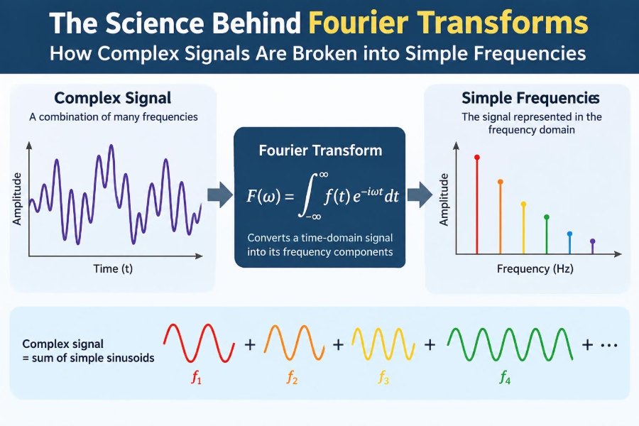
The core Fourier idea is that a sufficiently well-behaved signal can be represented as a combination of simple sinusoidal waves. Each component has a frequency, an amplitude, and a phase.
A sine wave is a smooth repeating oscillation. By adding many sine and cosine waves at carefully chosen strengths and alignments, engineers can reproduce remarkably complicated shapes, including speech fragments and non-repeating pulses over a measured interval.
The transform changes the question from “what is the signal doing at each instant?” to “which oscillatory components are present, and how strongly?”
🧭 Two complementary views of one signal
The original description is the time domain for a changing signal: voltage versus time, for example. The transformed description is the frequency domain: component strength versus frequency.
Neither view replaces the other. A time plot shows when an event occurred; a frequency plot shows its periodic structure. A sudden click is obvious in time, while a persistent 60 Hz electrical hum is often far clearer in frequency.
For images, the equivalent pair is space and spatial frequency. Broad gradual shading is low spatial frequency; fine stripes and sharp detail are high spatial frequency.
🌊 Why sine waves are the preferred building blocks
Sine and cosine waves have a special engineering advantage. When differentiated or integrated, they remain sine waves at the same frequency, with only their scale and phase changed.
They are also the natural responses of many linear physical systems. Springs, circuits, acoustic spaces, and control systems often respond to a sinusoidal input at that same input frequency, though with a changed amplitude and delay.
This makes frequency components easy to track through a system. A complicated input can be studied one frequency at a time and then recombined.
🧩 Fourier series for repeating patterns
A Fourier series applies when a signal repeats with a fixed period. It expresses that repeating waveform as a sum of a base frequency, called the fundamental, and integer multiples called harmonics.
A musical note from an ideal string is not generally a pure sine wave. Its fundamental helps establish perceived pitch, while harmonics help distinguish a flute-like tone from a bowed-string tone.
For a period T, the fundamental frequency is 1/T. The series asks how much of each harmonic frequency is needed to build one repeated cycle.
🔭 Fourier transforms for non-repeating signals
Real measurements often do not repeat neatly. A transient impact, a brief communication burst, or a single sensor record needs a continuous range of possible frequencies rather than only harmonic slots.
The Fourier transform extends the series idea by expressing a signal through a continuous frequency spectrum. Its inverse transform converts that spectrum back into the original signal.
Strict mathematical conditions can matter for unusual functions, but engineering uses the transform broadly for finite, sampled data. The practical question is whether the representation accurately serves the measurement and design task.
🔢 The role of complex numbers
Fourier transforms are usually written with complex exponentials such as e^(j2πft), where j denotes the square root of −1. This compact form represents sine and cosine together.
The complex result contains two pieces of information. Its magnitude indicates the strength of a frequency component, while its angle gives the phase, or alignment relative to a reference.
Complex numbers are not an optional mathematical decoration. They preserve timing relationships that magnitude alone cannot describe.
🕰️ Phase explains where waves line up
Two sine waves can have the same frequency and amplitude but reach peaks at different times. Their phase difference determines whether they reinforce one another, partly cancel, or form a shifted waveform.
Consider two loudspeakers playing the same tone. At some locations, their sound waves can arrive in phase and sound stronger; elsewhere, opposing phase can reduce the sound. The frequency content has not changed, but the spatial timing has.
Discarding phase can therefore make reconstruction impossible in general. A magnitude spectrum is useful, but it is not the complete signal description.
📊 Reading a spectrum without being misled
A spectrum commonly plots magnitude against frequency. Tall narrow peaks often indicate strong periodic components, while a broad spread may indicate noise, a transient, or rapidly changing behavior.
Always inspect axis units and scaling. Magnitude may be shown as linear amplitude, power, or decibels; frequency may be in hertz, radians per second, or normalized digital units.
A peak identifies a component in the measurement, not automatically its physical cause. A 120 Hz peak, for instance, may arise from a power-related mechanism, but diagnosis requires knowledge of the equipment and sensor path.
🎹 Harmonics, overtones, and waveform shape
A pure sinusoid has one frequency. A periodic but non-sinusoidal waveform contains harmonics. A square-like waveform needs many odd harmonics; sharper corners require significant energy at higher frequencies.
This relationship gives a practical interpretation of bandwidth. Fast changes and sharp transitions cannot be represented faithfully if high-frequency components are absent.
Harmonics are not automatically unwanted distortion. In audio they can be part of the desired timbre; in power electronics they may increase heating, interference, or torque ripple and therefore require control.
🧪 A simple two-tone example
Suppose a sensor signal is the sum of a 10 Hz vibration and a weaker 35 Hz vibration. Its time trace may look like one irregular wiggle, especially when the components overlap.
A Fourier transform produces peaks near 10 and 35 Hz. If the 35 Hz component grows over successive measurements, it can become a useful condition-monitoring clue even when the time waveform still looks confusing.
This is a hypothetical example, not a diagnostic rule. Real machines have multiple paths, changing loads, resonances, and noise that must be interpreted together.
🧱 Linearity makes decomposition work
The transform is linear: the transform of a sum is the sum of the transforms. If one signal is doubled, its transform is doubled; if two signals are added, their spectra add.
Linearity lets engineers separate analysis into manageable components. It also supports superposition in linear models, where individual sinusoidal responses can be calculated and combined.
Nonlinear systems complicate this picture. They can generate new harmonics, intermodulation products, and frequency shifts that were absent from the input.
⚙️ Convolution becomes multiplication
One of Fourier analysis’s most useful results is the convolution theorem. In the time domain, the output of a linear time-invariant system is often computed by convolution with its impulse response.
In the frequency domain, that same operation becomes multiplication: Y(f) = X(f)H(f). Here, H(f) is the system’s frequency response.
This explains why filters are naturally designed in frequency terms. A low-pass filter keeps low-frequency components relatively intact while reducing higher-frequency components.
🔁 The inverse transform is the reconstruction test
A transform is valuable because it is reversible under appropriate conditions. After changing, measuring, or selectively removing frequency components, the inverse Fourier transform synthesizes a time- or space-domain result.
For example, an audio editor may attenuate a narrow hum component in the spectrum and transform the result back to audio. The outcome depends on the filter design: removing too broad a range can damage wanted low-frequency content.
Reconstruction also reveals whether crucial information was discarded. Keeping only spectrum magnitude usually does not preserve the original waveform.
💻 The discrete Fourier transform
Computers do not receive continuous signals. They process finite sequences of samples. The discrete Fourier transform, or DFT, maps N samples into N frequency bins.
Each bin represents a particular discrete frequency component. For real-valued input data, the spectrum has a useful symmetry: negative-frequency information mirrors positive-frequency information in a complex-conjugate form.
That symmetry is mathematical, not a claim that physical negative-frequency vibrations are separately measured. It arises from the representation used for real signals.
⚡ Why the FFT changed engineering practice
The fast Fourier transform, or FFT, is an efficient algorithm for calculating the DFT. It produces the same transform values as a direct DFT calculation, but uses far fewer arithmetic operations for common data sizes.
The FFT made frequent spectral analysis practical in instruments, communications equipment, embedded systems, and scientific software. It is an algorithmic efficiency improvement, not a different transform.
Speed does not remove the need for sound setup. Sampling choices, scaling, windowing, and interpretation still determine whether an FFT result is meaningful.
📏 Sampling sets the usable frequency range
Sampling records a continuous signal at regular intervals. If the sample rate is fs, the highest frequency that can be represented without ambiguity is below the Nyquist frequency, fs/2.
The sampling theorem requires a rate greater than twice the highest frequency of interest for ideal band-limited signals. Physical signals are rarely perfectly band-limited, so practical acquisition systems use an analog anti-alias filter before sampling.
Sampling faster is not always better: it increases data volume and may expose noise outside the measurement need. The rate should match the required bandwidth and resolution.
🚨 Aliasing folds high frequencies into false low ones
Aliasing occurs when frequencies above the usable range masquerade as lower frequencies after sampling. Once sampled, the false component can be indistinguishable from a genuine low-frequency signal.
A rotating wheel in video can appear to slow, stop, or rotate backward when frame rate and rotation rate interact. That visual effect is a familiar aliasing example.
The remedy must occur before digitization: limit unwanted high-frequency content with analog filtering and choose a sufficient sample rate. A later digital filter cannot reliably identify and undo already-folded content.
🪟 Finite records create spectral leakage
An FFT analyzes a finite block of data. It effectively treats that block as one period of a repeated signal. If the first and last sample do not join smoothly, the artificial discontinuity spreads energy across nearby frequency bins.
This spreading is spectral leakage. A tone that lies between FFT bin frequencies may look wider and lower than expected, even with no physical change in the signal.
Leakage is a measurement effect, not necessarily noise or a fault. Understanding it prevents overinterpretation of small neighboring peaks.
🪟 Window functions trade leakage for resolution
Multiplying a record by a window that tapers at its ends reduces the artificial boundary jump. Common choices include Hann, Hamming, Blackman, and rectangular windows.
No window is universally best. Stronger sidelobe suppression can make a weak tone beside a strong tone easier to see, but it typically broadens the main spectral peak and reduces frequency discrimination.
| Choice | Useful tendency | Practical caution |
|---|---|---|
| Rectangular | Narrow main peak when cycles align | Can leak strongly when they do not |
| Hann | General-purpose leakage reduction | Broadens peaks compared with rectangular |
| Stronger taper | Suppresses distant sidelobes | Can merge closely spaced components |
🔍 Resolution is set mainly by observation time
For a record lasting T seconds, FFT bin spacing is approximately 1/T hertz. A longer observation provides finer frequency spacing because it watches more cycles.
Increasing the sample rate alone does not improve low-frequency bin spacing if the record duration stays fixed. It expands the measurable frequency range instead.
Zero-padding adds displayed frequency points between existing bins and can make a plot smoother. It does not create the resolving power of a longer measurement.
📉 Noise looks different after transformation
Random noise often distributes across many frequencies rather than appearing as one stable narrow line. Averaging spectra from repeated records can make persistent components easier to distinguish from random variation.
However, averaging can conceal intermittent events. If rare impacts are the engineering concern, time-domain inspection, triggered captures, or time-frequency methods may be more appropriate.
Noise treatment must serve the question. A display that looks cleaner is not automatically a measurement that is more truthful.
🎛️ Filters are frequency-selective decisions
Low-pass, high-pass, band-pass, and notch filters act on selected frequency ranges. They are used to remove drift, isolate a vibration band, suppress hum, or meet communication channel limits.
Every filter has trade-offs. A sharp transition can introduce delay, ringing, or phase distortion depending on the design. A notch filter can remove interference but may also remove nearby real information.
State the desired signal, undesired signal, acceptable distortion, and required timing before choosing a filter. “Remove noise” is not a complete specification.
📡 Communications use spectra to share space
Radio, Wi-Fi, cellular, and wired communication systems all rely on frequency-domain thinking. Information is placed into controlled frequency bands, shaped to limit interference, then recovered by receivers designed for those bands.
Modulation shifts information to a carrier frequency, while filtering confines transmitted energy and rejects unwanted channels. Fourier methods describe both the occupied bandwidth and the effects of transmission paths.
A sharp pulse in time tends to occupy broad bandwidth. This time-frequency trade-off is why rapidly changing signals require careful spectrum management.
🩺 Imaging and sensing turn frequency data into pictures
In medical imaging and scientific instruments, measured data may be acquired in a frequency-related domain and reconstructed using inverse transforms. Magnetic resonance imaging, for example, uses spatial-frequency data commonly called k-space in its reconstruction process.
Image processing also uses Fourier techniques for blur analysis, periodic-noise removal, and texture analysis. A blurred image has reduced high-spatial-frequency detail because fine edges have been weakened.
Transform methods do not bypass physical limitations. Sensor noise, incomplete data, motion, and model assumptions still affect reconstruction quality.
🏭 Vibration analysis finds repeating mechanical behavior
Rotating machinery commonly creates frequency components related to shaft speed, gears, blades, bearings, structural resonances, and electrical excitation. Spectra can help identify patterns that are hard to see in raw acceleration data.
A reliable analysis needs rotational speed, sensor placement, load condition, mounting quality, and baseline history. A frequency peak alone is evidence to investigate, not a complete failure diagnosis.
Trend changes over comparable operating conditions are often more informative than a single isolated spectrum.
🖼️ Images have two-dimensional frequency content
A two-dimensional Fourier transform decomposes an image into patterns varying across horizontal and vertical directions. Low frequencies describe broad illumination and large shapes; high frequencies describe fine detail and abrupt edges.
Periodic striping in an image can form distinct points in its two-dimensional spectrum, making targeted suppression possible. But aggressive frequency filtering can create halos or erase meaningful texture.
The same principle applies to spatial measurements in materials, optics, and fluid visualization: frequency is about rate of variation, not only sound.
⏱️ When one spectrum is not enough
An ordinary Fourier transform summarizes frequency content over the whole record. It cannot directly say when a brief frequency component appeared. A chirp and two separate tones can produce similar global frequency content.
The short-time Fourier transform analyzes overlapping short windows, creating a spectrogram with time, frequency, and intensity. Short windows improve timing information but reduce frequency resolution; long windows do the reverse.
Wavelet methods offer another approach for signals containing short transients across multiple scales. Choose the representation that matches the signal’s changing behavior.
🧮 Units and normalization prevent bad comparisons
FFT software packages differ in normalization. Some place the scaling in the forward transform, some in the inverse, and some split it. A raw FFT magnitude cannot be compared across settings unless scaling is understood.
Amplitude spectra, power spectra, and power spectral density answer different questions. Power spectral density is especially useful when comparing noise across different record lengths and frequency-bin widths.
Document sample rate, record length, window, averaging, sensor calibration, and amplitude convention with every result. A spectrum without metadata is difficult to reproduce or trust.
🛑 Common Fourier analysis mistakes
- Reading every peak as a real source: check leakage, aliases, harmonics, electrical pickup, and sensor resonances.
- Ignoring phase: magnitude-only plots cannot fully characterize waveform timing or reconstruction.
- Using an arbitrary window: choose it based on tone separation, amplitude accuracy, and signal conditions.
- Confusing zero-padding with resolution: longer duration, not extra zeros, separates close frequencies.
- Filtering before defining the objective: a visually smooth result may have lost the feature under investigation.
🧰 A disciplined workflow for real measurements
- Define the engineering question: detection, diagnosis, control, compression, or reconstruction.
- Estimate the frequency range and select sensor, anti-alias filtering, sample rate, and record duration.
- Inspect the raw signal for clipping, offsets, dropouts, and operating changes.
- Choose windowing, scaling, and averaging deliberately; retain the configuration.
- Interpret spectral features against physics, operating context, and repeat measurements.
- Validate conclusions with another measurement, condition, or model when consequences are significant.
This workflow treats the Fourier transform as part of an evidence chain rather than a button that delivers diagnoses.
🧠 The enduring Fourier principle
Fourier transforms work because complex behavior often becomes understandable when viewed as combinations of simple rates of change. They expose periodic structure, simplify linear-system calculations, and provide a bridge between measured signals and physical mechanisms.
The method has limits: finite records blur detail, sampling can create ambiguity, and a global spectrum can hide timing. Yet when acquisition and interpretation are handled carefully, the frequency domain reveals structure that the original waveform can conceal.
The essential lesson is simple: a Fourier transform does not change the signal—it changes the questions you can answer about it.
Whether you are analyzing sound, vibration, images, circuits, or communications, learn to move comfortably between time, space, and frequency. That shift in perspective is one of engineering mathematics’ most practical powers. 📐🌊⚙️