
A car’s suspension settles after hitting a pothole. A room gradually cools when its heater switches off. A phone battery drains faster during a video call than when it sits idle. These events look different, but each involves something changing over time.
Engineers need more than a snapshot of such systems. They need to estimate what happens next: whether a bridge will vibrate uncomfortably, whether a medicine pump will deliver the right amount, or whether a control system will remain stable after a disturbance.
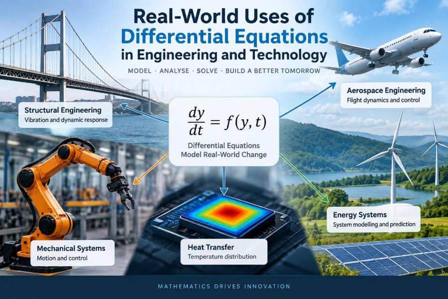
Differential equations provide a compact language for describing change. They connect a quantity—such as temperature, voltage, speed, population, pressure, or concentration—to the rate at which it changes.
That connection makes them central to engineering analysis, design, simulation, and control. The equations do not replace testing or professional judgement, but they help engineers reason about complex behavior before building expensive or safety-critical systems.
🧭 What a Differential Equation Actually Describes
A differential equation contains an unknown function and one or more of its derivatives. A derivative measures a rate of change: velocity is the rate of change of position, and acceleration is the rate of change of velocity.
For example, dT/dt = -k(T - Ta) states that an object’s temperature T changes at a rate proportional to the difference between its temperature and the surrounding temperature Ta. The constant k represents how quickly heat is exchanged.
The equation captures a rule of behavior, not merely a list of measured values. Once its parameters and starting conditions are known, it can predict a possible time history.
⏱️ Why Engineers Model Change Rather Than Just States
A static calculation can tell an engineer the force on a beam under a fixed load. It cannot, by itself, describe what happens when the load arrives suddenly, moves across the beam, or repeats thousands of times.
Many engineering failures and performance problems are dynamic. Overshoot in a motor controller, pressure surges in pipes, thermal cycling in electronics, and flutter in aircraft structures all depend on how conditions evolve.
Differential equations turn physical laws into dynamic models. They reveal not only the final condition but also the path taken to reach it, including delay, oscillation, instability, and transient peaks.
📏 The Role of Initial and Boundary Conditions
An equation alone rarely specifies one unique physical answer. Engineers also need conditions that describe the system at a particular time or location.
An initial condition gives a starting state, such as a tank initially containing 200 litres of water or a capacitor beginning at zero volts. A boundary condition specifies behavior at an edge, such as the fixed temperature at the ends of a metal rod.
These details are not administrative extras. Changing the initial charge on a capacitor or the boundary temperature of a wall can produce a completely different solution from the same governing equation.
🧱 Ordinary and Partial Differential Equations
An ordinary differential equation, or ODE, uses derivatives with respect to one independent variable, usually time. A mass on a spring, a rotating motor shaft, or a chemical concentration in a well-mixed reactor can often be modeled with ODEs.
A partial differential equation, or PDE, uses derivatives with respect to two or more variables. It is useful when behavior varies through both time and space, such as heat spreading across a circuit board or stress waves traveling through a structure.
| Model type | Typical variables | Example engineering use |
|---|---|---|
| ODE | Time | Motor speed response |
| PDE | Time and position | Heat flow through a wall |
| Coupled equations | Several interacting states | Vehicle dynamics and control |
The right choice depends on the question. If temperature differences across an object are negligible, one average temperature may be enough; if hot spots matter, a spatial PDE model is needed.
🌡️ Heat Transfer in Buildings and Devices
Thermal models are among the most familiar applications. A simple lumped model treats an object as having one uniform temperature and balances heat stored inside it against heat entering or leaving.
This approach helps estimate the warm-up of a water heater, the cool-down of a heated component, or the response of a thermostat-controlled room. More detailed PDE models describe conduction within walls, battery cells, heat exchangers, and semiconductor packages.
Thermal design often focuses on the highest temperature reached and the time spent near it. Excess temperature can shorten component life, degrade battery performance, or make a device unsafe to touch.
🔌 Electrical Circuits and Signal Behavior
Capacitors store electrical energy and resist sudden changes in voltage. Inductors store magnetic energy and resist sudden changes in current. These effects naturally lead to differential equations in resistor-capacitor and resistor-inductor circuits.
In an RC charging circuit, the capacitor voltage rises gradually rather than instantly. In an RLC circuit, voltage and current may oscillate, much like a mass attached to a spring.
Engineers use these models in filters, power supplies, sensor interfaces, radio-frequency systems, and timing circuits. They are especially useful for examining transients: short-lived events that can still damage components or corrupt signals.
🚗 Vehicle Suspension and Ride Comfort
A vehicle suspension must support the vehicle, reduce vibration, and keep tyres in contact with the road. A basic model combines mass, spring stiffness, and damping, producing a second-order differential equation.
If damping is too low, the car continues bouncing after a bump. If it is too high, the suspension can transmit sharp road inputs to occupants and reduce its ability to follow uneven terrain.
Real vehicle models add tyre flexibility, body pitch, roll, and changing loads. Even the simple model is valuable because it explains natural frequency, resonance, and the trade-off between comfort and road holding.
🏗️ Structural Vibration and Earthquake Response
Buildings, bridges, towers, and machine frames can vibrate when exposed to wind, traffic, rotating equipment, earthquakes, or sudden impacts. Their motion is governed by relationships among mass, stiffness, damping, and applied force.
A crucial question is whether the forcing frequency approaches the structure’s natural frequency. Near this condition, called resonance, vibration can become much larger than the original forcing might suggest.
Engineers use dynamic models to assess movement, fatigue, and occupant comfort. The model must represent connections, supports, material behavior, and loading realistically; a mathematically elegant model with poor assumptions can be misleading.
🌊 Fluid Flow in Pipes and Networks
Water distribution systems, oil pipelines, cooling loops, and process plants all involve changing flow and pressure. Differential equations express mass conservation, momentum balance, and energy losses.
One important transient is water hammer: a pressure wave caused by rapid changes in flow, such as a valve closing quickly. The pressure rise depends on system geometry, fluid properties, pipe elasticity, valve action, and other factors.
Models help engineers choose pipe sizes, pump controls, surge protection, and valve operating procedures. In complex networks, numerical simulation is usually necessary because flow paths and operating conditions interact.
✈️ Flight Dynamics and Aircraft Stability
An aircraft changes position, speed, orientation, and angular rate continuously. Differential equations connect aerodynamic forces and moments with translational and rotational motion.
Near a steady flight condition, engineers often linearize the equations: they approximate the system’s behavior for small deviations. This makes it possible to study modes such as pitch oscillation, roll response, and directional stability.
Linear models are powerful within their intended range, but they should not be treated as universal. Large maneuvers, stall conditions, and rapidly changing aerodynamic effects can require nonlinear models and extensive validation.
🛰️ Orbits, Satellites, and Spacecraft Motion
Orbital motion follows differential equations derived from gravitational attraction and Newton’s laws. A satellite’s acceleration changes continuously as its position relative to Earth changes.
For basic orbit prediction, a two-body model may be adequate. Mission planning can require additional effects, including atmospheric drag in low orbit, gravitational influences from other bodies, solar radiation pressure, and small propulsion maneuvers.
Spacecraft attitude control also uses differential equations. Reaction wheels, thrusters, and sensors must work together to point antennas, cameras, or solar panels accurately while avoiding unstable motion.
🤖 Robotics and Motion Planning
A robot arm is not simply a collection of rotating joints. Each link has mass and inertia, and movement at one joint can affect forces and accelerations throughout the mechanism.
Differential equations describe the robot’s dynamics, while kinematics describes its geometry and motion without considering forces. Both are needed when a robot must move quickly, carry a load, or interact safely with its environment.
Dynamic models support trajectory planning, motor sizing, vibration reduction, and collision response. In practice, uncertainty in friction, payload mass, and flexible components means controllers often combine model-based predictions with sensor feedback.
🎛️ Feedback Control Systems
Control engineering asks a practical question: how can a system automatically maintain a desired behavior despite disturbances? A thermostat, cruise control system, industrial furnace, and drone autopilot all use feedback.
A controller compares a measured output with a desired reference and adjusts an input. Differential equations describe the plant—the physical system being controlled—and the controller’s internal dynamics.
Feedback can reject disturbances, but poor tuning can cause slow response, excessive overshoot, sustained oscillation, or instability. A controller must be assessed across realistic operating conditions, not only for one ideal test case.
📈 Stability: Will a Disturbance Fade or Grow?
Stability is one of the most important questions differential equations can answer. If a small disturbance gradually disappears, the system is stable around that operating condition. If it grows, the system may move away from its intended state.
A ball resting at the bottom of a bowl is a useful analogy for stable behavior; a ball balanced on top of a hill represents an unstable equilibrium. Engineering examples include voltage regulators, aircraft motion, chemical reactors, and power networks.
Stability analysis does not remove every risk. It describes behavior within the model and the range of disturbances considered. Component saturation, delays, and unmodeled effects can alter real-world outcomes.
⚡ Electric Power Systems
Power grids must balance generation and demand continuously. Changes in load or generator output affect voltage, current, and system frequency, with dynamics occurring on multiple time scales.
Differential-algebraic equations are often used here. Differential parts describe evolving states such as machine rotor motion, while algebraic constraints represent instantaneous network relationships.
These models support studies of fault response, generator controls, grid-connected converters, and renewable-energy integration. They help engineers investigate whether the network can return to acceptable operation after a disturbance, subject to the assumptions and data used.
🔋 Batteries and Energy Storage
A battery is more complex than a fixed voltage source. Its terminal voltage depends on current, state of charge, temperature, internal resistance, and electrochemical processes.
Simple equivalent-circuit models use differential equations to represent effects such as voltage relaxation after charging or discharging. More detailed electrochemical models represent transport and reaction processes inside the cell.
The appropriate model depends on the task. A portable device may use a simple model for battery indication, while thermal management or cell-development work may demand much greater detail. Model complexity should earn its place by improving a real decision.
🧪 Chemical Reactors and Process Plants
In a chemical reactor, material enters, reacts, and leaves. Conservation laws produce equations for concentration, temperature, pressure, and volume. Reaction rates may depend strongly on temperature and reactant concentration.
Some reactions release heat. If heat removal cannot keep pace, temperature may rise, changing the reaction rate and creating a feedback loop. This is why process dynamics and control are essential to safe operation.
Engineers use models to design mixing, cooling systems, sensor placement, control strategies, and operating procedures. The kinetic expressions used in the model must be based on suitable experimental data, not assumed from a convenient formula.
💊 Medical Technology and Drug Delivery
Differential equations appear in biomedical engineering when a quantity changes inside the body or a medical device. A simplified pharmacokinetic model may describe how a drug enters the bloodstream, distributes among compartments, and is eliminated.
Infusion pumps use control principles to regulate delivery, while ventilators model airflow, pressure, and lung mechanics. These applications require special care because biological systems differ widely between individuals.
A model can inform design and monitoring, but it does not substitute for clinical validation, safety engineering, or qualified medical decision-making. Patient-specific conditions and device safeguards remain essential.
🌱 Population, Ecology, and Resource Management
Engineering projects can affect biological populations, water quality, and resource use. Differential equations can represent population growth, harvesting, pollutant decay, oxygen demand, or nutrient movement.
The familiar logistic growth equation introduces a carrying capacity, representing limits imposed by resources. It is useful as a conceptual model, but real ecosystems involve weather, migration, age structure, predation, and human activity.
For environmental planning, model outputs should be interpreted as conditional scenarios rather than certain forecasts. The greatest value often comes from identifying sensitive variables and comparing alternatives.
🌧️ Flood Forecasting and Drainage Design
When rain falls on a catchment, some water infiltrates the soil, some is stored temporarily, and some becomes runoff. Differential equations help represent these changing stores and flows.
Urban drainage design uses models to examine pipes, channels, detention basins, pumps, and surface flow paths. A short, intense storm can produce very different behavior from the same total rainfall spread over many hours.
Inputs are uncertain, especially future rainfall patterns and blocked-drain conditions. Sensible design therefore considers a range of scenarios, maintenance needs, and safe overflow routes rather than trusting one simulation result.
🏭 Manufacturing, Motors, and Industrial Machines
Production equipment contains many dynamic systems: servo motors positioning a cutting head, rollers controlling web tension, furnaces regulating temperature, and pumps maintaining flow.
A motor model links electrical current, electromagnetic torque, shaft speed, and mechanical load. This allows engineers to predict acceleration time, choose a drive, and tune a position controller.
Ignoring dynamics can lead to oscillatory motion, poor dimensional accuracy, excessive energy use, or premature wear. However, highly detailed models may be unnecessary for routine control tasks when a lower-order model captures the dominant behavior.
📡 Communications and Signal Processing
Many filters used in analog electronics are described directly by differential equations. They selectively reduce high-frequency noise, pass a desired frequency range, or shape a signal before conversion and transmission.
Engineers also use continuous-time models for phase-locked loops, amplifier dynamics, antenna-related circuits, and sensor conditioning. The time response matters because a filter that removes noise may also delay or distort rapid changes in the desired signal.
This is a recurring engineering trade-off: improving one performance measure can weaken another. Differential equations make those compromises visible before hardware is finalized.
🧩 Coupled Systems Reveal Hidden Interactions
Real systems rarely operate in isolation. An electric vehicle, for example, couples electrical power flow, battery temperature, motor torque, vehicle motion, and control software.
Coupled differential equations represent these interactions. A higher motor demand can increase battery current; increased current can raise heat generation; temperature can then influence resistance and available power.
Studying subsystems separately is still useful, especially early in design. But integrated modeling becomes important when interactions determine overall performance, safety margins, or control behavior.
🖥️ Analytical Solutions and Numerical Simulation
Some differential equations have exact analytical solutions written in familiar mathematical functions. These solutions are excellent for understanding general behavior and checking simple cases.
Many practical models are too nonlinear, too large, or too irregular for an exact closed-form solution. Engineers then use numerical methods, which calculate approximate values at small time or spatial steps.
Simulation results are approximations, not direct reality. Step size, solver choice, tolerances, and numerical stability can influence the answer, so numerical settings require the same engineering scrutiny as physical parameters.
🔍 Parameter Estimation and Model Calibration
Every model contains parameters: damping coefficients, heat-transfer rates, resistances, reaction constants, or material properties. Some can be measured directly; others must be inferred from test data.
Calibration adjusts uncertain parameters so that model behavior agrees reasonably with relevant observations. It should use data that represents the operating range of interest, not just one convenient experiment.
A close fit to past data does not automatically prove that a model is physically correct. Different parameter combinations can sometimes reproduce similar outputs, a problem known as identifiability. Independent measurements and simple models help reduce this risk.
✅ Verification and Validation Are Different Tasks
Verification asks whether the equations were solved and implemented correctly. It can include checking units, testing code against known solutions, and confirming that results converge when the numerical grid is refined.
Validation asks whether the model adequately represents the real system for its intended purpose. It involves comparison with suitable experiments, field measurements, or trusted operational data.
A model can be verified but invalid if its assumptions are unrealistic. Conversely, a model that happens to match one dataset may still contain coding errors. Both checks are necessary.
⚠️ Common Modeling Mistakes
The most damaging errors often occur before a solver is started. A model may omit a key mechanism, use inconsistent units, or assume a constant property that changes significantly with temperature or load.
- Confusing correlation with mechanism: a curve fit may predict nearby data but fail outside the measured range.
- Using ideal inputs: real sensors have noise, actuators have limits, and operating conditions vary.
- Ignoring uncertainty: one “best” parameter value can hide a wide range of plausible outcomes.
- Overcomplicating the model: extra states and parameters can make calibration difficult without improving decisions.
A useful model is not the one with the most equations. It is the one that answers a defined engineering question reliably enough for the decision being made.
🛠️ A Practical Workflow for Building Models
Good differential-equation models usually develop iteratively. Engineers begin with the purpose: predict temperature, assess stability, size a component, compare design options, or design a controller.
- Define the system boundary, inputs, outputs, and time or length scale.
- State assumptions clearly and choose the relevant conservation laws or physical principles.
- Derive equations, check dimensions, and select initial and boundary conditions.
- Estimate parameters from data, specifications, or targeted experiments.
- Simulate, compare against measurements, and revise the model where needed.
- Report limitations alongside the result, especially for safety-critical decisions.
Starting simple is usually wise. Complexity can be added when a discrepancy reveals that a neglected effect actually matters.
🎓 Skills That Make Differential Equations Useful
Solving textbook equations matters, but professional use requires a broader set of skills. Engineers must translate a physical situation into variables, balances, assumptions, and measurable parameters.
Useful habits include sketching the system, tracking units, estimating orders of magnitude, plotting results, and asking whether the predicted trend makes physical sense. Programming and numerical tools are valuable, yet they are most effective when paired with physical intuition.
Students can practice by modeling familiar systems: a cooling drink, a bicycle coasting downhill, a charging power bank, or water draining from a container. The key is to compare the model’s prediction with observation and explain any mismatch.
🔮 Digital Twins and Real-Time Engineering Models
A digital twin is a digital representation connected, to varying degrees, with data from a physical asset or process. Differential-equation models can provide its dynamic core, while sensors supply current conditions.
Applications may include monitoring equipment condition, predicting thermal loads, testing control changes virtually, or planning maintenance. The term does not guarantee accuracy; its usefulness depends on data quality, model suitability, and careful updating.
Real-time models often need to be simpler than design models because they must run quickly and robustly. This is another example of choosing fidelity to suit the job rather than pursuing maximum detail by default.
🧠 The Core Takeaway: Models Make Change Understandable
Differential equations appear across engineering because physical systems evolve. Forces change motion, temperature differences drive heat flow, voltage differences drive current, and concentration differences drive transport and reaction.
The same mathematical ideas—rates, accumulation, feedback, equilibrium, stability, and coupling—reappear in very different technologies. Recognizing that common structure allows engineers to transfer insight from circuits to mechanics, from thermal systems to chemical plants, and from vehicles to robotics.
The central discipline is not memorizing every solution method. It is choosing a model that is physically meaningful, matched to the decision, checked against reality, and honest about uncertainty.
Differential equations are powerful because they turn changing physical behavior into models that engineers can analyze, test, and improve. From a cooling device to a satellite, they help transform “what might happen?” into a question that can be examined carefully and responsibly. 📐⚙️🌍