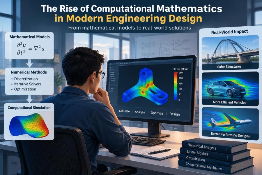

A bridge designer changes the thickness of a support by a few millimetres. An aircraft team adjusts the curve of a wing. A process engineer wants a heat exchanger to transfer more heat without creating an unacceptable pressure drop. None of these choices can safely be settled by visual intuition alone.
Physical prototypes remain valuable, but building and testing every possible version would be slow, expensive, and often impossible. Engineers therefore create mathematical representations of structures, fluids, heat, circuits, materials, and control systems before committing to hardware.
What has changed is the scale and speed at which those representations can now be solved. Computational mathematics turns equations that once required severe simplification into practical design tools, allowing engineers to explore alternatives, quantify uncertainty, and connect many physical effects in one workflow.
The result is not that mathematics replaces engineering judgment. Rather, it gives judgment a more detailed map: one that can reveal hidden loads, competing constraints, and consequences long before a product reaches the workshop or construction site.
🧭 What Computational Mathematics Means in Engineering
Computational mathematics is the use of mathematical models, numerical methods, and algorithms to solve problems with a computer. In engineering, it translates physical laws into calculations that estimate how a designed system will behave.
The term includes more than simulation software. It covers model formulation, discretization, optimization, data analysis, uncertainty estimation, and the careful interpretation of computed results. A colourful contour plot is only the visible end of a much larger mathematical process.
For example, a model of a bicycle frame may begin with equilibrium equations, material properties, geometry, and expected rider loads. Computational methods approximate the resulting stress field across the frame, helping the designer locate regions that deserve reinforcement or redesign.
📜 From Hand Calculations to Digital Models
Classical engineering mathematics relied heavily on closed-form solutions: formulas that provide an exact answer under idealized assumptions. Beam-bending equations and simple circuit laws remain essential because they are fast, transparent, and excellent for early estimates.
Real products, however, have irregular geometry, variable material properties, nonlinear behaviour, contact surfaces, turbulence, and changing operating conditions. These features rarely yield a neat analytical formula.
Digital computation made it practical to divide a difficult problem into many smaller, manageable pieces. This did not eliminate theory; it made advanced theory usable on geometries and conditions closer to those found in practice.
🧮 The Physical Model Comes First
A computation is only as meaningful as the model behind it. Engineers begin by deciding which physics matter: mechanics, heat transfer, fluid flow, electromagnetics, chemical reaction, or some combination.
They then specify inputs such as geometry, material behaviour, forces, boundary conditions, and initial conditions. A boundary condition might state that one edge of a plate is fixed, that a pipe inlet has a given flow rate, or that an electronic component dissipates a known amount of heat.
Leaving out a dominant effect can produce a precise-looking but misleading answer. For instance, modelling a metal component as perfectly elastic is inappropriate if expected loading may cause permanent deformation.
🔢 Why Numerical Methods Are Necessary
Most engineering models involve differential equations, which describe how a quantity changes across space or time. The heat equation describes the evolution of temperature, while the equations of motion describe displacement and acceleration.
Numerical methods replace a continuous problem with a finite set of approximate calculations. Instead of finding temperature at every imaginable point in a wall, a program calculates it at selected locations and estimates values between them.
This approximation is not a flaw to ignore; it is a controlled trade-off. The engineer must choose enough detail to answer the design question without consuming impractical computing time.
🕸️ Discretization: Turning Continuum into Pieces
Discretization is the step that divides a continuous object or process into discrete units. A structure can become a mesh of small elements, a fluid volume can become cells, and time can be represented as successive time steps.
Think of a high-resolution digital photograph. More pixels can represent a curved edge more faithfully, but they also create a larger file. In simulation, smaller elements can capture sharper stress changes or flow features, while demanding more memory and solver effort.
Discretization is a modelling decision, not an automatic guarantee of accuracy. The pieces must be appropriate in shape, size, and location for the physical phenomenon being studied.
🏗️ Finite Element Analysis for Solid Structures
Finite element analysis, often called FEA, is widely used for structures and mechanical components. It breaks a solid into connected elements and approximates displacement within each one. From displacement, the model estimates strain and stress.
FEA supports work on brackets, pressure vessels, building components, implants, machine frames, and many other systems. It is especially helpful where a geometry includes holes, fillets, joints, or load paths that make elementary formulas insufficient.
A stress concentration near a hole does not automatically mean failure. The engineer also needs material strength, fatigue behaviour, manufacturing detail, safety requirements, and realistic loading to decide whether the feature is acceptable.
🌊 Computational Fluid Dynamics and Moving Fluids
Computational fluid dynamics (CFD) solves approximate forms of the equations governing conservation of mass, momentum, and energy in liquids and gases. It can estimate pressure, velocity, temperature, and other flow properties through or around a design.
Applications include pump passages, ventilation systems, vehicle aerodynamics, combustion equipment, and process piping. A ventilation model, for example, may reveal stagnant zones where air exchange is poor or high-velocity regions likely to create noise.
Fluid models require particular caution because turbulence, multiphase flow, and flow separation can be difficult to represent. A CFD image can be informative, but its credibility depends on its assumptions and validation.
🔥 Heat Transfer Often Drives the Design
Thermal analysis predicts how heat moves by conduction, convection, and radiation. It matters in batteries, electronics, engines, buildings, industrial furnaces, and cryogenic equipment.
An electronic enclosure illustrates the interaction between mathematics and design. A model may show that a chip itself is within its temperature limit, while a nearby capacitor experiences a higher local temperature that could shorten its useful life.
Thermal performance is rarely isolated. Changing a heat sink shape can improve cooling but add mass, obstruct airflow, increase cost, or complicate assembly. Computational design is valuable precisely because it makes these coupled consequences visible.
⚡ Electromagnetic Models Beyond Circuit Diagrams
Circuit equations describe many electrical systems well, but components and fields become important when geometry, frequency, and spatial arrangement matter. Computational electromagnetics helps analyse motors, antennas, transformers, sensors, and high-speed electronic layouts.
A model may estimate magnetic flux in a motor or identify unwanted coupling between adjacent conductors. It can also help engineers understand where electrical fields are concentrated near sharp geometry.
Material data and operating conditions are crucial. Magnetic materials can behave nonlinearly, and electrical properties may change with temperature or frequency, so a simplified model must be matched to the purpose of the decision.
⏱️ Time-Dependent Simulation Reveals Transients
Some systems can be treated as steady: their relevant behaviour changes little with time. Others cannot. An impact event, a switching power supply, a startup sequence, or a sudden valve closure requires a time-dependent, or transient, analysis.
Time is broken into increments, and the model advances step by step. Very large increments can miss fast changes; extremely small increments can make a computation slow without providing useful additional information.
Choosing time resolution should follow the physical timescale of interest. A simulation of a slowly warming room and a simulation of a crash pulse demand very different temporal detail.
🔗 Multiphysics Connects Interacting Effects
Many design failures arise at the boundary between disciplines. A battery generates heat, temperature changes electrical behaviour, expansion creates mechanical stress, and deformation can alter electrical contact. Treating each effect separately may conceal the feedback loop.
Multiphysics simulation couples two or more physical models. Common combinations include fluid-structure interaction, thermal-stress analysis, electromagnetic heating, and electrochemical-thermal battery models.
Coupling should be used when the interaction materially affects a decision. It is not automatically better than a simpler model; added complexity introduces additional assumptions, input requirements, and possibilities for numerical difficulty.
🎯 Optimization Changes the Design Question
Analysis asks, “How does this design behave?” Optimization asks, “Which allowed design is best according to stated objectives?” The difference changes the workflow from evaluating a single candidate to searching a design space.
An optimization problem requires objectives, design variables, and constraints. A lightweight bracket might minimize mass while limiting stress, displacement, and manufacturing restrictions. The solver evaluates alternatives and directs the search toward promising regions.
There is rarely one universally best answer. A shape with minimum mass may be harder to manufacture, less robust to uncertain loads, or more expensive. Clear objectives prevent an apparently sophisticated optimization from pursuing the wrong outcome.
🧩 Design Variables, Constraints, and Trade-offs
Design variables are quantities the engineer is permitted to change: thickness, diameter, material selection, control gains, fin spacing, or geometric coordinates. Constraints define what must remain true, such as a maximum temperature, minimum safety margin, or fixed installation envelope.
Some projects have competing objectives. Improving fuel efficiency may conflict with acceleration, while reducing pressure loss may require a larger component. Rather than hiding that conflict, computational methods can map a set of viable compromises.
This is often called a Pareto trade-off: moving toward a better result in one objective requires accepting a worse result in another. Decision-makers can then choose deliberately rather than assuming a single numerical score captures every value.
🧱 Topology Optimization and Manufacturable Shapes
Topology optimization distributes material within a permitted region to achieve a target such as stiffness at low mass. The results can look organic because the method identifies efficient load paths rather than following conventional geometric habits.
Such output is a starting point, not always a production drawing. Thin members, enclosed voids, unsupported overhangs, tolerances, inspection access, and joining requirements may make the raw shape unsuitable for manufacturing.
A productive workflow applies manufacturing rules during optimization or redesigns the result afterward. The mathematical optimum and the practical engineering solution must meet in the same component.
📊 Data Enters the Engineering Loop
Computational mathematics increasingly works alongside measured data from sensors, tests, manufacturing systems, and operational equipment. Data can estimate uncertain parameters, detect deviations, or update a model as a system ages.
A pump model, for instance, may be compared with measured pressure and flow data to determine whether performance has shifted from its expected condition. The model offers structure; measurements provide evidence about the real system.
Data alone does not explain causation, and models alone do not guarantee realism. Combining them carefully is often more useful than treating either as a complete substitute for the other.
🪞 Digital Twins Are Models with an Operational Role
A digital twin is generally understood as a digital representation connected, to some meaningful degree, with a real asset or process. The connection may involve design information, live sensor inputs, historical data, or updates based on inspections.
For a wind turbine, a twin might track operating loads and environmental conditions to support maintenance decisions. For a factory process, it may help compare expected and observed performance.
The label should not be used loosely. A static CAD model is useful, but it is not automatically a digital twin. The operational connection and the purpose of the representation matter.
🤖 Machine Learning Has a Focused Role
Machine learning can find patterns in large datasets, estimate expensive model outputs, classify defects, or create fast surrogate models for optimization. A surrogate is an approximation trained to imitate a more costly simulation within a defined range.
It is particularly useful when thousands of design evaluations would otherwise be required. But a model trained on limited or biased data may fail outside the conditions it has seen.
Physics-based constraints, sound test data, and clear uncertainty checks remain necessary. Machine learning is a useful computational component, not a replacement for conservation laws, engineering requirements, or accountability.
✅ Verification Checks Whether the Equations Were Solved Correctly
Verification asks whether the computational implementation correctly solves the chosen mathematical model. It concerns numerical error, programming or setup mistakes, mesh quality, solver settings, and convergence.
Common checks include refining the mesh, reducing the time step, monitoring residuals, and comparing simple cases against known analytical solutions. If a result changes substantially as the mesh is refined, the original mesh may have been too coarse.
Convergence deserves careful interpretation. A solver reporting convergence means its iterative process met a mathematical criterion; it does not prove that the model represents the real device accurately.
🔬 Validation Checks Whether the Model Represents Reality
Validation compares model predictions with appropriate physical measurements or trusted reference data. It asks a different question: are the assumptions and inputs suitable for the actual system and intended use?
A structural model can be numerically flawless yet invalid if it assumes a rigid support where the real connection is flexible. Similarly, a thermal model may miss a contact resistance at an interface and underpredict local temperatures.
Validation should match the application. A model intended for early design screening may need less detailed evidence than one used to support a high-consequence operational decision, but neither should be accepted merely because the images look plausible.
📏 Mesh Independence and Resolution Discipline
Mesh refinement is one of the most practical safeguards in computational work. Engineers compare results across progressively finer meshes to determine whether key outputs—such as peak stress, pressure loss, or natural frequency—have stabilized sufficiently.
Resolution should be concentrated where gradients are high: near contacts, sharp geometry changes, boundary layers, heat sources, or expected crack locations. Uniformly making every region tiny is often inefficient.
A peak value at a mathematically sharp corner may rise as the mesh is refined because the idealized geometry creates a singularity. In that case, the useful response is not simply to report an ever-larger number, but to examine the physical radius, material behaviour, and design-relevant stress measure.
⚠️ Boundary Conditions Can Dominate the Result
Boundary conditions often have more influence than the choice between two reasonable solver options. A force applied at the wrong location, an unrealistic fixed support, or an assumed uniform temperature can redirect the entire solution.
Before running a large model, ask basic physical questions: Where does the load come from? How is it transferred? What can move? Where does heat leave? Which quantities are measured and which are assumed?
Simple free-body diagrams, hand estimates, and discussions with test or manufacturing teams frequently expose weak assumptions early, when corrections are inexpensive.
🧪 Experiments Remain Essential
Simulation can reduce the number of physical prototypes, but it cannot remove the need for testing. Experiments reveal material variability, assembly effects, unmodelled interactions, and real-world misuse that no early model fully captures.
Testing and computation are most powerful as a loop. Test results calibrate and validate models; models then help choose the next test condition, instrument location, or design variation worth investigating.
For safety-critical systems, the required evidence depends on the application, governing requirements, and consequences of failure. A simulation is evidence within an engineering case, not an automatic certificate of safety.
💻 Solver Choice Shapes Cost and Reliability
Different mathematical formulations and solvers suit different problems. Some methods solve all unknowns together; others iterate toward a solution. Explicit time integration can suit short, highly dynamic events, while implicit approaches are often efficient for slower structural response.
The right choice depends on nonlinearity, scale, accuracy needs, available computing resources, and the question being asked. A sophisticated solver cannot compensate for unsuitable inputs, while an unnecessarily elaborate method can delay useful design feedback.
Engineers benefit from understanding the basic assumptions of their software rather than treating it as a black box. Knowing what a tool approximates makes warnings and unexpected results easier to investigate.
☁️ Computing Power Expands the Search Space
Parallel computing, cloud resources, and improved numerical libraries allow teams to run larger models and explore more alternatives than a single workstation could reasonably handle. This is especially useful for parameter sweeps, uncertainty studies, and optimization.
More computing power does not remove the need for model discipline. It can just as easily produce thousands of unverified results faster. Computing budgets should be directed toward decisions where better resolution or broader exploration will alter the engineering choice.
Reproducible workflows also matter. Recorded model versions, input data, solver settings, and post-processing steps help teams trace why a result changed and allow colleagues to review the work.
🧑🤝🧑 Collaboration Makes Models More Credible
Modern engineering models cross disciplinary boundaries. A mechanical analyst may need material data from a specialist, operating loads from a systems engineer, dimensions from a CAD designer, and test evidence from a laboratory team.
Clear communication prevents false precision. Reporting assumptions, load cases, limits, and uncertainty is more useful than presenting a final number without context.
A good review question is, “What decision does this result support?” It keeps the team focused on the relevant output and makes it easier to spot analysis that is technically elaborate but operationally disconnected.
🚫 Common Failure Modes in Simulation Work
Several mistakes appear repeatedly, especially when software is accessible before modelling fundamentals are secure:
- Trusting a polished visualisation without checking units, mesh, or boundary conditions.
- Using material properties from an inappropriate temperature range, condition, or source.
- Applying loads as idealized points when the real contact area matters.
- Reporting a single result without examining sensitivity to uncertain inputs.
- Optimizing a model before verifying that it represents the intended physical problem.
These are not merely technical oversights. They can lead to wasted prototypes, misplaced confidence, or a design that performs differently from its prediction.
🛠️ A Practical Workflow for Better Decisions
A dependable computational workflow is iterative rather than linear. Start with the simplest model capable of answering the immediate question, then increase fidelity only when the decision demands it.
- Define the design decision, performance measures, and acceptable limits.
- Build a conceptual model using governing physics and defensible assumptions.
- Perform hand calculations or scaling estimates to establish expected ranges.
- Create the numerical model, then verify mesh, time resolution, and solver behaviour.
- Validate against relevant evidence where possible and document remaining uncertainty.
- Use results to compare alternatives, revise the design, and plan targeted tests.
This sequence makes analysis a learning process, not a final-stage approval ritual.
🎓 Skills Engineers Need Alongside Software
Effective users of computational mathematics need more than menu familiarity. They need calculus, linear algebra, differential equations, probability, mechanics or domain physics, and enough programming literacy to automate checks and manage data.
They also need modelling judgment: the ability to simplify responsibly, recognize unreasonable outputs, and explain assumptions to non-specialists. A rough estimate performed on paper remains one of the best checks on a complex digital result.
For students, small reproducible models are a strong starting point. Solve a beam problem analytically, model it numerically, refine the mesh, and compare the answers. The comparison teaches more than pressing “run” on a large template.
🌱 Sustainability Benefits from Quantified Trade-offs
Computational design can support lower material use, improved energy efficiency, reduced waste, and longer service life. For example, an engineer can compare insulation thicknesses by balancing heat loss against material use and space constraints.
Environmental conclusions still require a full system view. Reducing mass might lower operational energy demand but require a material with more intensive processing, difficult recycling, or shorter durability.
Mathematical models make such trade-offs easier to examine, but they do not assign social priorities. Those priorities must be made explicit by engineering teams, clients, regulators, and communities where relevant.
🔐 Responsible Use Includes Transparency
As design decisions become more automated, traceability becomes more valuable. Teams should be able to state which inputs were used, what conditions were considered, where the model is reliable, and what it does not cover.
Access to powerful tools also raises practical questions about proprietary data, cybersecurity, and ownership of model outputs. These are engineering-management concerns as much as software concerns, particularly for connected operational models.
Responsible computational practice resists both extremes: neither dismissing models as unreliable nor treating them as unquestionable authority.
🚀 Where Computational Mathematics Is Heading
Engineering workflows are becoming more connected across design, simulation, manufacturing, testing, and operation. Faster solvers, reduced-order models, automation, and data-informed updates will continue to shorten the path from question to informed comparison.
The lasting challenge is not simply generating more results. It is selecting the right level of model complexity, preserving traceability, and ensuring that predictions remain tied to physical evidence and a real engineering decision.
In that sense, the future belongs to engineers who can move comfortably between first principles, computation, data, and practical constraints.
🧠 The Core Principle: Use Computation to Improve Judgment
Computational mathematics has changed modern engineering design because it exposes behaviour that is difficult, costly, or unsafe to observe directly. It enables engineers to test alternatives, understand interactions, and locate critical conditions before they become physical surprises.
Its strength does not lie in producing the most detailed model possible. Its strength lies in creating a model that is fit for purpose, checked against mathematics and reality, and used transparently alongside testing and professional judgment.
The best computational result is therefore not the most dramatic visualisation or the longest report. It is the result that helps a team make a better, better-supported design decision.
Modern engineering design advances when mathematics, computation, measurement, and human judgment are treated as complementary parts of the same discipline. That combination turns numerical power into safer, more useful, and more responsible engineering. 📐💻🔧