
A flow meter records water moving through a pipe every second. A vehicle test logs speed at regular intervals. A temperature sensor samples heat in a furnace. Each dataset gives engineers separate values, but the question they often need answered is about the total: total volume, distance travelled, or energy transferred.
When the underlying relationship is known exactly, calculus supplies an integral. In practice, however, engineers frequently have measurements rather than a neat formula. Even when a formula exists, it may be too complicated to integrate conveniently by hand.
Numerical integration turns a collection of values into a reliable estimate of accumulated quantity. It is one of the quiet workhorses of engineering analysis, simulation, testing, and design.
The calculations can be simple, but choosing a method, spacing data sensibly, and recognizing error require engineering judgment. This is where numerical integration becomes more than “adding up values.”
🧩 The central idea: accumulation from pieces
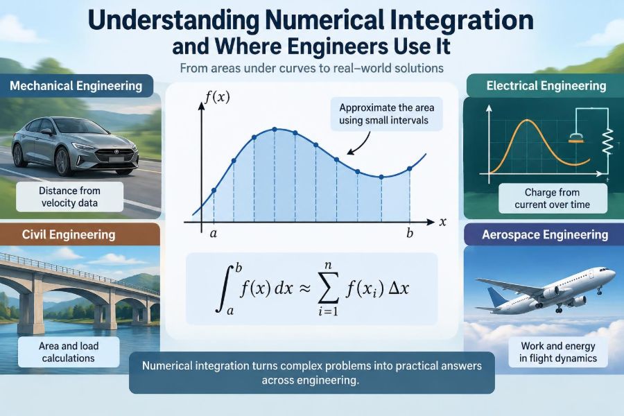
Integration adds infinitely many tiny contributions. If a force varies as an object moves, the work done is the accumulated contribution of force over each tiny distance. On a graph, it is the signed area between the curve and the horizontal axis.
Numerical integration replaces the unknown tiny pieces with a finite set of manageable pieces. It approximates the area under sampled data or a computed function across an interval.
📈 Reading an integral on a graph
For a function y = f(x), the definite integral from a to b is written ∫[a,b] f(x) dx. Its units are the units of f(x) multiplied by the units of x.
If velocity is measured in metres per second and time in seconds, integrating velocity over time produces metres. Checking units is one of the quickest ways to spot a mistaken setup.
🧱 Why exact calculus is not always available
An analytical integral is an exact expression found using calculus rules. It is ideal when the equation is known and has a tractable antiderivative.
But a wind-tunnel sensor does not deliver a symbolic equation for pressure. A finite-element model may provide values only at mesh points. Some functions also have antiderivatives that cannot be expressed using elementary functions. Numerical methods remain useful in all of these cases.
📊 Discrete data is the usual engineering starting point
A sampled dataset contains pairs such as (t, v), (x, p), or (T, q). Numerical integration estimates the total response between the first and last sample.
For example, a pump test may report flow rate every minute. Adding the estimated flow-volume contribution from each minute gives the fluid volume moved during the test. This is not merely a mathematical convenience; it connects logged operating data to a physical total.
🪜 The rectangle rule: the first approximation
Divide an interval into strips of width h. The rectangle rule treats the function height in each strip as constant, so the estimated integral is the sum of rectangle areas.
Using the left endpoint gives h[f(x₀)+f(x₁)+...+f(xₙ₋₁)]. Using the right endpoint shifts every chosen height one sample forward. A midpoint version uses the value halfway through each strip and is often more accurate for smooth functions.
↔️ Left, right, and midpoint choices
For an increasing function, left rectangles tend to underestimate area and right rectangles tend to overestimate it. The reverse occurs for a decreasing function. This behavior can provide a useful rough error bracket when the trend is monotonic.
Midpoint rectangles better represent gradual curvature because the sample is centered in each interval. They do require either midpoint measurements or an ability to calculate values there.
🔺 The trapezoidal rule follows the data
The trapezoidal rule joins neighboring points with straight lines rather than holding each interval flat. The area from xᵢ to xᵢ₊₁ is approximated by (xᵢ₊₁ − xᵢ)[f(xᵢ)+f(xᵢ₊₁)]/2.
For equally spaced values, it becomes h[f(x₀)/2 + f(x₁) + ... + f(xₙ₋₁) + f(xₙ)/2]. It is widely used because it works directly with ordinary tabulated data and is exact for any straight-line trend.
🧠 A small velocity example
Suppose a vehicle’s speed is measured as 10 m/s at one second and 14 m/s one second later. Assuming speed changed linearly over that interval, the trapezoidal estimate of distance is 1 × (10 + 14)/2 = 12 m.
This estimate is not claiming the car truly accelerated uniformly. It states the assumption used to fill in information between two measurements. More frequent samples reduce dependence on that assumption when the motion changes rapidly.
〰️ Simpson’s rule uses curved segments
Simpson’s rule approximates the curve with quadratic polynomials over pairs of equal-width intervals. For an even number of intervals, the composite form is h/3[f₀ + 4f₁ + 2f₂ + 4f₃ + ... + 2fₙ₋₂ + 4fₙ₋₁ + fₙ].
The alternating weights may look unusual, but they arise from integrating fitted parabolas. For sufficiently smooth, equally spaced data, Simpson’s rule can achieve much lower approximation error than the trapezoidal rule with the same interval width.
⚖️ Choosing between common rules
| Method | Best fit | Main limitation |
|---|---|---|
| Rectangle | Quick estimates and teaching the concept | Can miss slope and curvature |
| Trapezoidal | Measured data, including uneven spacing | Sensitive to strong curvature between samples |
| Simpson’s | Smooth values at equal spacing | Requires interval-count and spacing conditions |
| Adaptive quadrature | Computer evaluation of known functions | Does not repair an incorrect model |
No method is universally “best.” The appropriate choice depends on whether values are measured or calculated, how smooth the behavior is, and what uncertainty the decision can tolerate.
🧮 Unequal spacing needs careful treatment
Real sensor timestamps are not always evenly separated. Data may be missing, a logger may drift, or an event-triggered system may sample more often during rapid change.
The trapezoidal rule handles this naturally: calculate each interval using its own width. Applying the standard equally spaced Simpson formula to uneven data is not valid. Interpolation or a method designed for irregular points may be needed instead.
🎯 What numerical integration error means
Numerical error is the difference between the estimated integral and the true integral of the underlying function. It comes from representing a curved or changing quantity with simple shapes.
Error usually decreases as intervals become narrower for a well-behaved function, but “smaller” is not the same as “known to be acceptable.” Measurement noise, sensor bias, and model uncertainty may be much larger than the approximation error.
🌊 Curvature and abrupt changes are warning signs
Widely spaced samples can miss a narrow pressure spike, a switching transient, or a rapidly changing load. A smooth-looking plot may simply be a consequence of joining sparse points.
Where sharp features are physically plausible, engineers sample more densely near those features or use adaptive algorithms that place extra evaluation points where the function appears difficult to approximate.
🔍 Refining the mesh as an error check
A practical computational check is to integrate with a chosen spacing, then repeat using smaller spacing. If the answer changes materially, the original discretization was too coarse for the required result.
This is called a convergence check. It does not prove correctness, especially if the physical model is wrong, but it tests whether the numerical approximation is stabilizing.
🧪 Noise can become accumulated uncertainty
Measurements contain random variation and may include offsets. Integration often smooths high-frequency random noise to some extent, but a persistent offset accumulates directly into the total.
A flow meter that reads slightly high over a long batch will overestimate volume. Before integrating, engineers may need calibration checks, filtering appropriate to the signal, and a clear record of how missing or rejected data were handled.
🚗 Motion analysis: velocity, acceleration, and distance
Vehicle dynamics provides a familiar chain of integrations. Integrate acceleration over time to estimate change in velocity; integrate velocity over time to estimate displacement.
Inertial sensors are valuable but prone to drift. A tiny acceleration bias can produce a growing velocity error and an even larger position error after repeated integration. Numerical technique matters, but sensor correction and reference measurements matter just as much.
💧 Flow and volume in process systems
Chemical plants, water networks, and manufacturing lines often measure volumetric or mass flow rate. Integrating the rate over time gives the amount transferred, consumed, or produced.
Engineers must keep the basis consistent. A volumetric flow rate may depend on temperature and pressure, while mass flow is often preferable for material balances. Integrating accurate numbers with mismatched physical definitions still gives the wrong operational answer.
⚡ Electrical energy from power data
Electrical power changes with load. Integrating power over time gives energy, which supports battery analysis, equipment testing, and consumption monitoring.
If power is in watts and time is in seconds, the integral is joules. If power is in kilowatts and time is in hours, the result is kilowatt-hours. Unit conversions should be made explicit before values are summed.
🏗️ Structural work and strain energy
When a material or structure deforms, the area under a force-displacement curve represents work. Likewise, the area under a stress-strain curve represents energy per unit volume under the applicable loading interpretation.
Test machines generate discrete readings, so engineers numerically integrate the curve. Care is needed around unloading, hysteresis, and permanent deformation: different portions of the curve can represent stored recoverable energy or dissipated energy.
🌡️ Heat transfer and cumulative exposure
A varying heat-transfer rate integrated over time gives total heat transferred. This appears in thermal cycling, heat-exchanger trials, and energy balances for equipment that does not operate at steady state.
Temperature history can also matter when materials or products respond to cumulative exposure. The correct integrand may be a temperature-dependent rate rather than temperature itself, so selecting the physical model comes before selecting a numerical rule.
🌬️ Fluid mechanics and distributed loads
Pressure is rarely uniform over a curved surface, and velocity profiles vary across a pipe or channel. Integrating a pressure distribution can yield resultant force; integrating a velocity profile over cross-sectional area yields flow rate.
Computational fluid dynamics often supplies values at many mesh locations. Numerical integration converts these local predictions into engineering quantities such as drag, lift, torque, and mass flow.
🛰️ Simulation outputs need integration too
Many simulation tools solve differential equations by stepping through time. Their output may include instantaneous force, current, temperature, or reaction rate. Post-processing these histories often requires numerical integration.
A simulation result is not automatically more accurate because it contains thousands of points. Time-step selection, solver tolerances, and the validity of the underlying equations all influence whether an integrated output is credible.
🗺️ Finite elements and integration over space
Integration is not only over time. In finite element analysis, quantities are integrated across lengths, areas, and volumes to form stiffness matrices, calculate loads, and recover total energy.
Software commonly uses Gaussian quadrature, which evaluates a function at carefully chosen points and weights them to integrate polynomials efficiently. Users do not always see these calculations, but mesh quality and element formulation affect their reliability.
💻 Spreadsheets and code reduce arithmetic, not judgment
A spreadsheet can implement the trapezoidal rule by calculating interval widths, averaging adjacent values, and summing the resulting areas. Scientific programming libraries offer integration routines, including adaptive methods for functions that can be evaluated on demand.
Automation prevents repetitive arithmetic errors, but it can conceal setup errors. Plot the raw signal, inspect units, identify gaps, and retain the data-processing assumptions alongside the final total.
🧾 A reliable workflow for tabulated data
- Define the accumulated quantity and its expected units.
- Inspect timestamps or spatial locations for ordering, gaps, and unequal spacing.
- Plot the values to identify outliers, steps, and regions of rapid change.
- Select a method consistent with data spacing and expected smoothness.
- Calculate the integral and perform a units and magnitude check.
- Test sensitivity by refining data where possible or comparing a second reasonable method.
- Document filtering, interpolation, calibration, and assumptions.
This workflow makes the result reviewable. In engineering, an answer that cannot be traced back to its data and assumptions is difficult to trust.
🚫 Common mistakes that distort totals
- Ignoring nonuniform intervals: treating every sample as if it had the same width changes the weighting of the data.
- Mixing units: seconds, minutes, watts, and kilowatts can produce large conversion errors.
- Interpolating across an event: a straight line through a valve opening or machine shutdown may not represent the actual behavior.
- Double-counting endpoints: interval methods have specific endpoint weights.
- Integrating a biased signal without correction: small offsets can dominate a long-duration total.
🧭 Interpolation is an assumption, not a measurement
Integration methods implicitly interpolate between known values. Trapezoidal integration assumes straight segments; Simpson’s rule assumes local parabolic behavior. More elaborate splines can create smooth curves, but smoothness is not evidence that the curve is physically correct.
Use interpolation that matches the process knowledge. A discontinuous control signal may need to be treated as piecewise constant, while a slowly varying thermal signal may reasonably support a smooth approximation.
🧷 Signed area versus total magnitude
An ordinary integral is signed: values below zero subtract from values above zero. This is essential for net displacement, net charge, or net flow direction.
Sometimes the desired quantity is total activity regardless of direction, such as total path length from velocity or total vibration measure from an alternating signal. In those cases, integrate the magnitude or use a separately defined metric. The question determines the integrand.
🛠️ Matching precision to the decision
Not every task warrants a sophisticated method. A preliminary estimate may need only a transparent trapezoidal calculation, while design verification or performance acceptance may require denser instrumentation, uncertainty analysis, and independent checks.
More decimal places do not imply more knowledge. Report a precision that is justified by the data quality and the intended engineering decision.
🎓 Building intuition through simple tests
Before trusting a workflow on complex data, test it on cases with known answers. A constant signal should integrate exactly with any sensible rule. A linear signal should integrate exactly with the trapezoidal rule.
These checks reveal indexing mistakes, incorrect interval widths, and unit-conversion errors quickly. They also build intuition for what each method is approximating.
✅ The core takeaway: integrate the physics, not just the numbers
Numerical integration estimates accumulated physical effects from functions or measured samples. Rectangles, trapezoids, Simpson’s rule, and adaptive methods differ in how they represent behavior between points.
The dependable result comes from combining an appropriate algorithm with sound data, correct units, sensible sampling, and a model that matches the process. A polished calculation cannot recover information a sensor never captured or correct an invalid physical assumption.
Numerical integration is most valuable when it turns trustworthy local information into a total that engineers can explain, check, and use to make decisions. With that mindset, areas under curves become distances, volumes, energies, forces, and practical engineering insight. 📐⚙️📊