
A test rig is running, a spreadsheet is filling up, and the values do not land on a perfectly straight pattern. Load increases with deflection, voltage rises with current, or pressure changes with flow—but every reading is slightly different from the neat relationship expected in theory.
That is normal. Experimental engineering data contain measurement uncertainty, small changes in operating conditions, instrument limits, and sometimes genuine physical effects. The challenge is not to force the readings to look ideal. It is to extract a useful model without hiding what the data are saying.
Fitting a straight line is one of the most practical ways to do this. A line can summarize a trend, estimate an unknown parameter, support calibration, and provide a basis for prediction within a tested range.
The method is simple in principle, but good line fitting depends on sound choices before, during, and after the calculation. The numbers matter; so do the axes, units, residuals, and engineering judgment behind them.
🧭 What fitting a straight line means
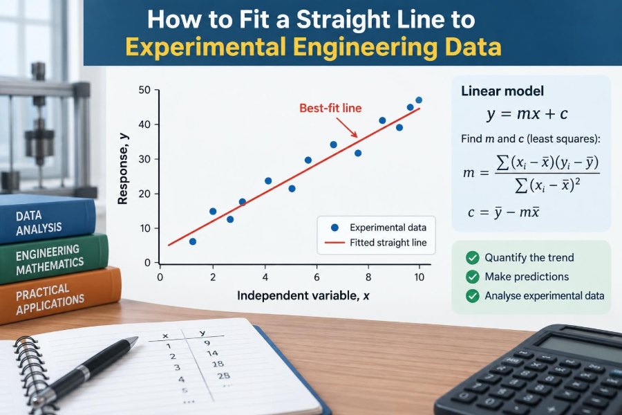
To fit a straight line is to find a linear equation that represents the overall relationship between two measured variables. The usual form is y = mx + c, where m is the gradient and c is the intercept.
The fitted line is usually not expected to pass through every point. Instead, it represents the central trend of the data as well as possible according to a chosen fitting rule.
🔧 Why engineers use linear models
Many engineering relationships are linear over a useful operating range, even when they are not linear everywhere. A metallic strain gauge, for example, may produce an output approximately proportional to strain over its specified range.
A line also turns observations into parameters with physical meaning. Its gradient may be stiffness, sensitivity, resistance, thermal expansion rate, or a calibration factor. The intercept can reveal an offset, a zero error, or a meaningful baseline condition.
📈 Start with a scatter plot
Plot the measured pairs before calculating anything. Put the independent or controlled variable on the horizontal axis and the response variable on the vertical axis, unless the physical problem gives a clear reason to do otherwise.
A scatter plot can immediately reveal curvature, separate operating regimes, an outlying point, or a transcription error. A formula alone cannot tell you whether a straight-line model is sensible.
🎯 Identify the independent and dependent variables
The independent variable, commonly written as x, is the quantity deliberately varied or treated as the input. The dependent variable, y, is the observed response.
In a beam test where known loads are applied and deflection is measured, load is normally x and deflection is y. This convention makes the gradient represent deflection per unit load. Reversing the axes changes the equation and the interpretation of its parameters.
📏 Check units before fitting
Units are part of the model, not decoration on a graph. If y is temperature in degrees Celsius and x is electrical power in watts, the gradient has units of degrees Celsius per watt.
Check whether unit conversions are needed before entering data into a calculator or spreadsheet. Mixing millimetres and metres, or kilopascals and pascals, can create a numerically convincing but physically wrong result.
🧪 Know when a straight line is plausible
A linear fit is appropriate when equal changes in x produce roughly equal changes in y across the range being used. It is an approximation to local behaviour, not a claim that nature always follows a line.
For example, a spring may follow Hooke’s law over modest extension, while material yielding makes the load-extension curve change shape. Fitting one line across both regions would conceal the transition engineers need to notice.
📝 Prepare a clean data table
Keep raw readings separate from processed values. A useful table includes run number, x, y, units, and notes about unusual conditions such as a restarted test or an instrument reset.
Do not round readings aggressively before fitting. Small rounding changes can noticeably affect a gradient when the measured range is narrow. Retain reasonable precision in the calculation and round the reported result at the end.
🧮 The equation of the fitted line
The standard engineering form is y = mx + c. The gradient m gives the change in predicted response for one unit change in input, while the intercept c is the predicted value of y when x = 0.
Neither parameter should be treated as merely a mathematical output. Ask whether its sign, units, and magnitude make sense for the apparatus and the theory being tested.
📐 Estimate a line by eye for understanding
Drawing a reasonable line through the middle of a scatter plot is a useful first check, especially in laboratory work. It helps detect a calculator entry error and builds intuition about the expected gradient.
Choose two well-separated points on the drawn line, rather than two noisy measured points, and calculate m = (y₂ − y₁)/(x₂ − x₁). This graphical estimate is educational, but it is subjective and rarely the best final method.
⚖️ The least-squares principle
The most common formal method is ordinary least squares. It chooses m and c so that the sum of the squares of the vertical differences between the measured points and the line is as small as possible.
Those vertical differences are called residuals. Squaring them prevents positive and negative deviations from cancelling, and it gives larger discrepancies more influence than smaller ones.
➕ Calculate the least-squares gradient
For n data pairs, the ordinary least-squares gradient is:
m = [nΣ(xy) − (Σx)(Σy)] / [nΣ(x²) − (Σx)²]The expression works when the x values are not all the same. If they are, there is no horizontal spread from which to estimate a gradient.
➖ Calculate the intercept
Once the gradient is known, calculate the intercept with:
c = [Σy − mΣx] / nAn equivalent and often more intuitive form is c = ȳ − mx̄, where x̄ and ȳ are the sample means. This shows that an ordinary least-squares line passes through the point (x̄, ȳ).
🧾 Work through a small hypothetical example
Suppose a calibration test gives approximately 1.2 V, 2.1 V, 3.1 V, and 4.0 V at inputs of 1, 2, 3, and 4 units respectively. The points are close to a line with a gradient near 0.94 V per input unit and a small positive intercept.
The resulting model might be reported as V = 0.94x + 0.25, subject to the exact calculation. Its meaning is practical: each added input unit increases predicted output by about 0.94 V, while the 0.25 V intercept suggests an offset worth investigating.
🖥️ Use spreadsheet tools carefully
Spreadsheets can calculate a linear regression quickly, plot a trendline, and display the equation. They are valuable because they reduce arithmetic effort and make it easy to update results when a data point is corrected.
However, software does not validate the experiment. Confirm that the selected columns are correct, that headers have not been included as data, and that the chart is an XY scatter plot rather than a category-based line chart.
💻 Reproduce the calculation in code
Code is useful when data sets are large, repeated tests must be processed consistently, or uncertainty analysis is required. The logic should remain transparent: read the data, inspect the plot, fit the model, calculate residuals, and report parameters with units.
# conceptual pseudocode
m, c = linear_least_squares(x, y)
y_fit = m*x + c
residual = y - y_fit
A reliable workflow stores raw data unchanged and creates a separate analysis output. That makes results easier to audit and reproduce.
🧩 Interpret the gradient physically
A gradient is often the engineering result of greatest interest. On a force-versus-extension graph, its reciprocal or direct value may relate to compliance or stiffness, depending on which variable is plotted vertically.
Always state the units beside the number. Saying “the slope is 3.2” is incomplete; saying “the sensitivity is 3.2 mV/N” communicates a measurable property.
🚦 Treat the intercept with caution
An intercept is sometimes physically required. A sensor may have a genuine output at zero input, or a thermal system may have a baseline temperature above zero power because of ambient conditions.
But an intercept can also result from zeroing error, fixture preload, background signal, or extrapolation beyond the measured range. If no readings exist near x = 0, do not overstate what the fitted intercept proves.
📍 Understand residuals
For each data point, the residual is measured y − predicted y. A positive residual lies above the fitted line; a negative residual lies below it.
Residuals are more informative than a graph of raw points once a model has been fitted. They show where the line systematically misses the data and help separate random scatter from a flawed model.
🔎 Read a residual plot
Plot residuals against x or against fitted values. For a suitable linear model, they should generally form an unstructured cloud around zero with a roughly consistent spread.
A curved residual pattern suggests that the relationship is not adequately linear. A widening fan shape suggests that variability increases with the signal level, which affects how confidently one uniform-error model can be used.
📊 Use R² without worshipping it
The coefficient of determination, R², describes how much of the variation in the observed y values is represented by the fitted linear model under the calculation’s assumptions. Values closer to 1 often indicate a closer fit to the observed data.
R² is not proof that the model is physically correct. A high value can occur over a narrow range, with many points, or even for a relationship whose small curvature is not yet obvious. Inspect the plot, residuals, and physical mechanism as well.
⚠️ Recognize an outlier before deleting it
An outlier is a point that differs substantially from the surrounding pattern. It may be caused by a recording mistake, a loose connection, a missed equilibrium condition, or a real but unusual physical event.
Never remove a point simply because it weakens the fit. First check test notes, instrument status, units, and repeatability. If a point is excluded, document the reason and, where useful, show how its inclusion changes the result.
🪤 Watch for high-leverage points
A point far from the mean x value has high leverage: it can strongly influence the line’s gradient even if its vertical residual is not dramatic. A single reading at the edge of the test range deserves particular scrutiny.
This is not an argument for removing edge points. Well-measured extremes are often valuable because they establish the usable range. The lesson is to collect enough data across the range rather than relying on one influential observation.
🔬 Distinguish random scatter from bias
Random scatter makes repeated readings vary unpredictably around a trend. Taking repeat measurements can help estimate that variability and reduce the influence of any one reading on the fitted line.
Bias shifts readings consistently in one direction, perhaps through an uncalibrated sensor or systematic zero error. More repeats do not remove bias. Calibration checks, reference measurements, and improved procedures are needed instead.
⚙️ Know the assumptions behind ordinary least squares
Ordinary least squares is most straightforward when uncertainty in x is small compared with uncertainty in y, observations are reasonably independent, and the vertical scatter is of broadly similar size across the range.
Real experiments only approximate these conditions. The method can still be useful, but its limitations should guide interpretation—especially when both axes have substantial measurement error or when readings are collected in a time-dependent sequence.
⚖️ Use weighted fitting when precision changes
Some instruments are more precise in one part of their range than another. If individual measurements have known and meaningfully different uncertainties, weighted least squares can give more reliable readings greater influence than noisier ones.
The weights should come from a defensible uncertainty estimate, not from a desire to make the line look better. When uncertainty information is unavailable, ordinary least squares may be a reasonable practical choice, provided the limitation is acknowledged.
🔄 When errors exist in both variables
In many physical experiments, neither axis is exact. Fitting vertical residuals alone then assigns all measurement error to y, which may distort the estimated relationship if uncertainty in x is substantial.
Methods such as orthogonal regression or errors-in-variables fitting can be more appropriate because they account for uncertainty in both coordinates. They require assumptions about relative uncertainties, so they should be selected for a reason rather than used automatically.
🧱 Do not force a line through the origin casually
It can be tempting to impose c = 0 because theory suggests zero input should give zero output. This changes the fitting problem and can noticeably alter the gradient.
Constrain the intercept only when the zero condition is physically justified and the measurement system supports it. If the instrument has a zero offset, forcing the line through the origin transfers that offset into the slope and produces a biased calibration.
🌀 Recognize nonlinear behaviour
A curved scatter plot may indicate saturation, friction, heat transfer effects, geometric nonlinearity, chemical change, or a threshold process. A poor linear fit is sometimes the most useful finding because it identifies where the simple model stops applying.
Possible next steps include fitting an appropriate nonlinear model, transforming variables when theory supports it, or fitting separate linear sections for distinct operating regimes. Do not transform data merely to improve appearance; preserve a physical reason for the choice.
🗺️ Avoid extrapolation beyond the tested range
Interpolation estimates a value between measured inputs and is usually safer than extrapolation, which extends the fitted line beyond the available data. A straight trend can bend, saturate, or fail outside the experiment’s range.
State the calibration or validity range alongside the equation. A model fitted from 10 to 50 N should not quietly be used to predict 200 N without separate evidence that the same relationship remains valid.
📋 Report a fitted line professionally
A useful engineering report makes the result checkable. Include the model equation, variable definitions, units, data range, fitting method, graph, and a brief comment on residual behaviour or uncertainty.
- State whether the intercept was fitted freely or constrained.
- Use sensible significant figures; do not report more precision than the measurements support.
- Describe exclusions and unusual points transparently.
- Separate a fitted empirical relationship from a theoretical law.
This context lets another engineer decide whether the model is suitable for design, monitoring, calibration, or only preliminary analysis.
✅ A practical line-fitting workflow
- Define the input and response variables, including units and expected mechanism.
- Record clean raw data and relevant test conditions.
- Plot an XY scatter graph and look for range, curvature, and anomalies.
- Fit an unconstrained least-squares line unless a justified constraint applies.
- Check gradient, intercept, residuals, and the physical plausibility of the result.
- Investigate unusual points rather than deleting them automatically.
- Report the valid range and avoid unsupported extrapolation.
This workflow is quick enough for routine laboratory analysis while remaining rigorous enough to expose problems before a model is used in a decision.
🏁 The core principle of fitting experimental data
A straight line is not a way to make imperfect measurements look perfect. It is a compact model that should preserve the central trend while leaving evidence of uncertainty, offsets, and model limitations visible.
The strongest analysis combines calculation with observation: plot first, fit thoughtfully, inspect residuals, and interpret parameters in their physical context. When those steps agree, the fitted line becomes a useful engineering tool rather than just an equation generated by software.
Fit the line to understand the experiment—not to hide the experiment. A transparent model, stated with its range and limitations, is far more valuable than a tidy equation with no engineering judgment behind it. 📐📊🔧