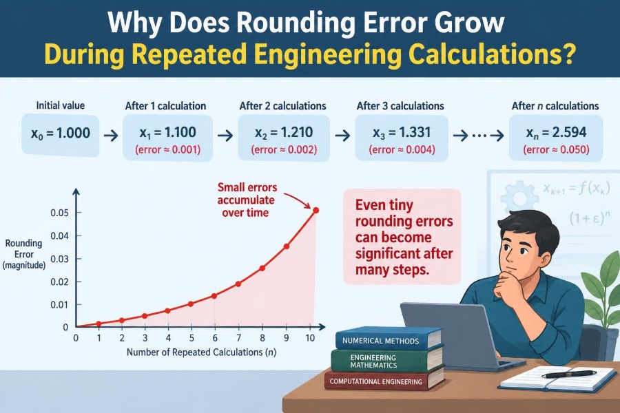

A spreadsheet predicts a pump’s energy use. A simulation advances a vehicle’s position one tiny time step at a time. A control system repeatedly converts sensor readings, applies a formula, and sends a command.
Each calculation may look harmless when viewed alone. The displayed answer might even be rounded to a reassuring number of decimal places. Yet after thousands, millions, or billions of operations, a small numerical discrepancy can become visible—or can quietly change a design decision.
This is not usually a sign that mathematics has failed. It is a consequence of asking finite digital hardware to represent an effectively continuous world. Engineering calculations need approximations, but those approximations have to be managed.
Understanding why error grows helps engineers choose suitable data types, algorithms, tolerances, tests, and reporting precision. It also prevents a common mistake: blaming “rounding” when the larger problem is actually a poorly conditioned model or an unstable computational method.
🔢 The basic meaning of rounding error
Rounding error is the difference between an exact mathematical value and the nearby value retained by a calculation system. It appears whenever a number has more digits than the chosen representation can store.
If a quantity is recorded as 1.23 rather than 1.23456, the difference is rounding error. A computer does the same kind of shortening, though usually in binary rather than decimal and with far more stored digits than a hand calculation.
The error can be positive or negative. That direction matters because errors sometimes cancel, but they can also reinforce one another.
💻 Why computers cannot store most real numbers exactly
There are infinitely many real numbers between any two values. A computer has a finite number of bits, so it can represent only a finite set of numbers in any chosen format.
Most engineering software uses floating-point numbers: a sign, a scaled significand, and an exponent. This efficiently handles very large and very small magnitudes, but it leaves gaps between representable values.
Numbers such as 0.1, 1/3, and many measured constants have repeating binary expansions. They are stored as close approximations, not exact values. The approximation is normally tiny, but repeated use gives it opportunities to matter.
🧮 Decimal intuition can be misleading
In base ten, one third is 0.333… and cannot be written with a finite number of decimal digits. In base two, the same issue affects many familiar decimals.
For example, a program may store a value intended as 0.1 slightly above or below the mathematical 0.1. Adding that stored value ten times need not produce the exact stored representation intended for 1.0.
This does not mean computers are unreliable. It means equality and precision need to be treated as numerical questions, rather than as assumptions based on how a number is printed.
📏 Absolute error and relative error answer different questions
Absolute error is the raw difference between approximation and exact value. If a computed length is 10.002 m instead of 10.000 m, the absolute error is 0.002 m.
Relative error scales that difference by the size of the true value. An error of 0.002 m is negligible for a kilometre-scale route but substantial for a small precision component.
Repeated calculations can enlarge either measure. Engineers should choose the one tied to the requirement: a permitted displacement, a percentage calibration deviation, or a safety margin, for example.
🎯 One calculation can introduce several errors
Rounding is only one source of numerical discrepancy. Input measurements have uncertainty, physical models simplify reality, numerical methods approximate equations, and output values may be rounded again for reporting.
These sources should not be casually added together as though they are identical. Measurement uncertainty describes limited knowledge of a physical quantity, while floating-point rounding describes a computational representation limit.
Still, they interact. Excessive numerical noise can conceal a genuinely small physical effect, while an overly precise printout can imply confidence that the measurements do not support.
🔁 Repetition creates an accumulation path
A repeated calculation feeds one result into the next. This occurs in running totals, numerical integration, iterative solvers, control loops, optimization routines, and time-stepping simulations.
Suppose a program updates a tank volume by adding flow multiplied by a short time interval. If each update has a tiny rounding discrepancy, the next update starts from the already approximated volume.
Error therefore has a path through the calculation. It is not merely a collection of isolated, invisible differences.
➕ Summing many values is the simplest example
Adding a long sequence is a familiar source of accumulated rounding error. Every addition rounds its intermediate result to a representable number.
When all terms are of similar magnitude, the effect may remain modest. When a huge running total receives many tiny increments, the increments can become difficult to retain because the spacing between nearby floating-point values grows with magnitude.
A tiny correction may then be rounded away entirely. This is especially relevant when a simulation accumulates small changes over a large baseline quantity.
⚖️ Error does not always grow in a straight line
It is tempting to say that each operation adds one more error of the same sign. Real calculations are less tidy. Some errors cancel, some behave like fluctuating noise, and some become correlated.
For a well-behaved process, aggregate error may grow more slowly than a worst-case sum. But relying on accidental cancellation is not a design strategy.
A systematic bias—such as always truncating downward—can produce roughly one-directional drift. Feedback and instability can amplify even irregular errors far more quickly.
✂️ Truncation introduces directional bias
Truncation drops digits rather than selecting the nearest representable value. If values are consistently cut toward zero or toward a lower bound, the errors have a preferred direction.
Consider repeatedly charging a usage total in a system that always truncates each small charge downward. The final total tends to underestimate the unrounded result. In engineering, similar bias can distort accumulated energy, mass, distance, or timing.
Round-to-nearest is generally less biased for ordinary floating-point operations, although it does not remove the need for error analysis.
🧱 Intermediate results matter more than displayed results
A report may show three decimal places, while the software retains much more precision internally. That is usually desirable: rounding only at final presentation avoids injecting unnecessary error into every subsequent step.
The reverse practice—rounding each intermediate value to match a report—is a frequent spreadsheet and hand-calculation mistake. It turns a display convention into a computational limitation.
Keep working values at appropriate internal precision, then round the final answer in a way consistent with the required tolerance and measurement uncertainty.
🔍 Subtracting close numbers can destroy useful digits
Catastrophic cancellation occurs when two nearly equal numbers are subtracted. Their leading digits cancel, leaving a small result whose remaining digits may be dominated by prior rounding error.
For instance, estimating a tiny difference between two large, nearly equal pressure values can be far less accurate than either pressure separately. The subtraction itself is mathematically valid; the representation makes the result fragile.
Algebraic reformulation can help. A standard example is replacing an expression such as sqrt(x+1)-sqrt(x) with the equivalent 1/(sqrt(x+1)+sqrt(x)) when x is large.
📉 Dividing by a small quantity magnifies uncertainty
Division by a small value can turn a modest absolute input error into a large output error. This is not uniquely a floating-point problem; it is a property of the mathematical relationship.
For example, calculating a parameter from a ratio becomes sensitive when its denominator approaches zero. Rounding error is then amplified alongside measurement error and model uncertainty.
Before treating a surprising result as a software defect, inspect the formula’s sensitivity near the operating condition.
🌊 Recurrence relations can amplify tiny differences
A recurrence defines the next value from prior values. This makes it central to dynamic simulations and digital control. If the recurrence is stable, small disturbances tend to remain bounded or decay.
If it is unstable, tiny discrepancies—including ordinary rounding—can grow rapidly. Two runs that differ only in arithmetic order or hardware settings may eventually diverge.
Divergence does not automatically mean either run represents physical reality. It may reveal that the discrete method, step size, or model is unsuitable for the requested time horizon.
⏱️ Time-step simulations face two separate errors
Numerical simulations often replace continuous time with increments such as 0.01 s. This introduces discretization error: error from approximating a continuous equation with finite steps.
Floating-point rounding occurs on top of that. Reducing the time step may reduce discretization error, but it also increases the number of arithmetic operations and therefore the opportunities for rounding effects.
The best step size is not simply “as small as possible.” It must balance method accuracy, stability, computational cost, and the precision relevant to the engineering decision.
🧭 Order of operations changes a floating-point answer
Real-number addition is associative: mathematically, (a+b)+c equals a+(b+c). Floating-point addition may produce slightly different results because each intermediate sum rounds.
This explains why a parallel program, a different compiler setting, or a rearranged spreadsheet can produce a different final digit. The difference is often harmless, but it can complicate reproducibility and testing.
For sensitive workloads, define deterministic reduction order where practical, and judge agreement using an appropriate tolerance rather than demanding bit-for-bit identity without reason.
🧠 Conditioning describes sensitivity in the problem itself
A problem is well-conditioned when small changes in inputs cause proportionally small changes in outputs. It is ill-conditioned when tiny input changes can produce much larger output changes.
Conditioning belongs to the mathematical problem, not the software implementation. Estimating the intersection of nearly parallel lines, fitting highly correlated parameters, and inverting a nearly singular matrix can all be ill-conditioned.
Better arithmetic cannot fully rescue a question that is intrinsically sensitive. It may reduce computational error, but it cannot create information absent from the inputs.
🛠️ Stability describes the algorithm
Stability concerns how an algorithm handles small disturbances during its own execution. A stable method does not needlessly magnify the errors it encounters; an unstable one can.
This distinction is essential. A stable algorithm applied to an ill-conditioned problem may still give a sensitive answer. An unstable algorithm can perform badly even on a problem that is otherwise well-conditioned.
When diagnosing error growth, ask two questions: is the underlying problem sensitive, and is the chosen computational procedure amplifying that sensitivity?
📐 Matrix calculations reveal hidden amplification
Engineering models often solve systems of linear equations. A matrix with a large condition number can amplify small changes in coefficients or right-hand-side values into large changes in the solution.
Directly computing a matrix inverse is frequently less desirable than solving the system with a suitable factorization. Methods such as pivoted elimination or QR-based approaches are designed to improve numerical behaviour in many settings.
The right method depends on matrix structure, scale, sparsity, and accuracy needs. There is no single numerical recipe that is best for every model.
🧪 A simple running-total thought experiment
Imagine adding one million small increments to a large total. In exact arithmetic, the final total is independent of the grouping of additions. In finite arithmetic, grouping can affect how many small increments survive rounding.
Adding from smallest magnitude to largest often preserves more small contributions than adding them into a very large partial total. This is a useful intuition, not a universal replacement for analysis.
For critical totals, use compensated summation or a carefully designed reduction method rather than assuming an ordinary loop is accurate enough.
🧷 Compensated summation retains lost low-order bits
Compensated summation keeps a small correction term that estimates the low-order information lost in previous additions. The correction is fed back into later additions.
It costs more operations than a naive sum, but can significantly improve accuracy when summing values with very different magnitudes. Variants include Kahan-style and pairwise summation approaches.
This is a good example of a broader principle: numerical accuracy often improves through algorithm design, not merely through requesting more decimal places.
🗃️ Precision choices have practical trade-offs
Single precision stores fewer significant bits than double precision, so it has larger spacing between representable numbers at a given scale. Double precision is often a sensible default for general engineering computation, but it is not infinite precision.
Higher precision can reduce rounding effects, yet it uses more memory, bandwidth, and processing time. On some systems, these costs affect simulation scale or real-time performance.
Choose precision from an error budget and operating range. A sensor cannot justify arbitrary computational precision if its uncertainty is much larger, but a long iterative calculation may still require more precision than its raw inputs suggest.
💱 Fixed-point arithmetic has a different set of risks
Fixed-point formats represent values in fixed increments, such as thousandths. They can be valuable for deterministic embedded applications, currency-like quantities, and systems with carefully bounded ranges.
The trade-off is limited range and explicit scaling. Overflow, underflow, and scaling mistakes can be more dangerous than the rounding issue the format was intended to control.
Fixed point is not automatically more accurate than floating point. It is appropriate when its quantization step, range, and deterministic behaviour match the application.
🧯 Overflow, underflow, and loss of significance
Rounding error is not the only finite-arithmetic hazard. Overflow occurs when a value exceeds the format’s representable range. Underflow occurs when a nonzero value is too small to be represented normally.
Loss of significance can occur before either limit is reached, particularly when combining vastly different scales or subtracting close values. A result may be finite and look plausible while retaining fewer meaningful digits than expected.
Range checks, dimensional scaling, and diagnostic logging help expose these problems early.
📊 Scaling variables improves numerical behaviour
Equations mixing quantities around 10-9 with quantities around 109 are harder to handle than equivalent equations expressed near comparable scales. This does not change the physics; it changes the numerical landscape.
Nondimensionalization and sensible engineering units can reduce extreme coefficient ranges. In matrix problems, scaling rows and columns may improve practical solution behaviour.
Scaling must be tracked carefully. A numerically tidy calculation is only useful if units and physical interpretation are restored correctly at the end.
✅ Tolerances are better than exact equality tests
Testing whether two floating-point values are exactly equal is often unsuitable when they were obtained through different sequences of operations. A tiny final difference can be expected even when both computations are valid.
Use a tolerance tied to the application. A combined absolute and relative test is common: absolute tolerance handles values near zero, while relative tolerance scales with magnitude.
A tolerance should never be a vague large number chosen only to make tests pass. It should reflect physical requirements, model sensitivity, and expected numerical error.
🧾 Report precision honestly
More printed digits do not create more trustworthy information. A value such as 14.237891 may be appropriate for an internal diagnostic, but a design report should use precision supported by input quality and the decision being made.
Conversely, rounding too aggressively can conceal threshold crossings or make independent checks impossible. Keep full internal results when needed, record assumptions, and state tolerances or uncertainty where they affect interpretation.
Clear reporting distinguishes computational resolution from physical accuracy.
🔬 Test calculations with known cases
Verification asks whether code solves the implemented equations correctly; validation asks whether those equations represent the intended physical system adequately. Rounding analysis belongs primarily to verification, but affects both.
Useful checks include simplified cases with known answers, conservation balances, limiting cases, unit tests for sensitive expressions, and comparisons across precision levels or step sizes.
If a result changes materially when using a more stable summation order or a finer resolution, that change is evidence to investigate—not automatically proof that the newest result is correct.
🚩 Common responses that do not solve the problem
Several habits sound reasonable but can leave the root cause untouched:
- Rounding every intermediate result “to keep it neat.”
- Switching to higher precision without checking conditioning or stability.
- Using exact equality in tests for independently computed floating-point results.
- Making time steps smaller without assessing method stability and total error.
- Ignoring unit scale, range limits, and near-zero denominators.
The remedy must match the mechanism. An ill-conditioned formulation needs reformulation or better information; an unstable method needs a different algorithm or step strategy.
🧰 A practical workflow for engineering calculations
Start by defining what accuracy means for the decision. Is the limit an absolute displacement, a relative force error, a pass/fail threshold, or a control-loop timing requirement?
- Estimate the expected range and scale of all quantities.
- Separate measurement uncertainty, model approximation, discretization error, and arithmetic rounding.
- Select precision and algorithms suited to that range and sensitivity.
- Avoid unnecessary intermediate rounding and fragile algebraic forms.
- Test convergence, conservation, and sensitivity to reasonable computational changes.
- Document tolerances, units, assumptions, and any remaining limitations.
This workflow makes numerical reliability a design activity rather than an emergency debugging task.
🏗️ When rounding error is genuinely consequential
Many ordinary engineering calculations have error margins so large that floating-point rounding is negligible. Spending weeks optimizing the last binary digit would be wasted effort.
It deserves closer attention when calculations are long-running, iterative, poorly scaled, near a threshold, highly sensitive, safety-related, or required to be reproducible across systems. Embedded control, large simulations, optimization, navigation, and financial-like accounting components can have particularly different needs.
The criterion is consequence, not curiosity. Focus analysis where a realistic numerical discrepancy could alter an operational, design, compliance, or safety decision.
🧩 The core principle: small errors meet sensitive processes
Rounding error grows during repeated engineering calculations when finite representations are repeatedly introduced, carried forward, and sometimes amplified by the mathematics or the algorithm. Repetition alone is not the whole story.
Growth is most troublesome when there is systematic bias, loss of small terms, cancellation, division by small quantities, an ill-conditioned problem, or an unstable recurrence. Good numerical practice addresses each mechanism directly.
Engineers do not need perfect arithmetic to make dependable decisions. They need calculations whose remaining error is understood, bounded where possible, and small compared with the tolerance that actually matters.
Rounding error becomes manageable when representation, algorithm, scale, and engineering tolerance are treated as one connected problem. 📐🔧