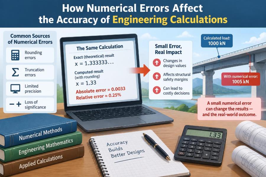

A design spreadsheet returns a beam deflection of 4.98 mm. A simulation gives 5.01 mm. A sensor report shows 5.0 mm. At first glance, the three values seem to tell the same story.
But suppose the allowable deflection is 5 mm. Now the last decimal place is no longer cosmetic. It can affect whether an engineer investigates the model, changes a section size, repeats a measurement, or accepts a result.
Engineering calculations turn physical reality into numbers, and every step in that translation has limits. Instruments have finite resolution, material properties vary, data are rounded, and computers store only a finite set of digits.
Numerical errors do not automatically make a calculation useless. The real skill is understanding where error enters, how it travels, and whether it is large enough to change a decision.
🎯 Accuracy is not the same as precision
Accuracy describes closeness to the true value. Precision describes how closely repeated values agree with one another. A set of measurements can be precise but inaccurate if they cluster around the wrong value.
Imagine a pressure gauge that consistently reads 3 kPa too high. Its readings may be repeatable, yet they are biased. Conversely, readings scattered around the true pressure may have low precision even if their average is accurate.
🧭 The “true value” is often an ideal
In textbooks, error is often written as the difference between an approximate value and a true value. In practice, the true value may be unavailable. A bridge load, soil stiffness, or heat-transfer coefficient can change with conditions and cannot always be known exactly.
Engineers therefore compare against a reference: a calibrated instrument, a higher-fidelity model, a carefully controlled test, or an accepted design value. Error analysis is usually about estimating credible uncertainty, not claiming perfect knowledge.
📏 Absolute error gives the size of a difference
Absolute error is the magnitude of the difference between an approximate result and a reference value:
absolute error = |approximate value − reference value|If a calculated flow rate is 1.97 m³/s and the reference is 2.00 m³/s, the absolute error is 0.03 m³/s. This is useful when the units themselves matter, such as millimetres of displacement or degrees of temperature.
🔢 Relative error puts the difference in context
A 0.03 m³/s error is interpreted differently for a small laboratory flow than for a major river channel. Relative error compares the discrepancy with the reference magnitude:
relative error = absolute error / |reference value|Multiplying by 100 gives percentage error. Relative measures are especially helpful when comparing errors across variables with different scales, but they become unstable when the reference value is close to zero.
🧪 Measurement error begins before calculation
Many engineering computations start with measured inputs: dimensions, temperatures, voltage, mass, pressure, speed, or strain. If an input is uncertain, no later arithmetic can make it exact.
Consider calculating resistance from voltage and current. A highly accurate formula does not compensate for a current sensor with drift or an incorrectly chosen measurement range. The model inherits the quality of its inputs.
📐 Instrument resolution limits what can be seen
Resolution is the smallest change an instrument can display or distinguish. A digital caliper that displays to 0.01 mm does not prove that every reading is accurate to 0.01 mm; it only limits the displayed increment.
Resolution matters most when the expected change is similar in size to the instrument step. Reporting a temperature change of 0.003°C from a device that displays tenths of a degree suggests detail the instrument did not provide.
⚖️ Calibration errors create systematic bias
A systematic error shifts results consistently in one direction. Typical causes include a sensor with a zero offset, an incorrectly calibrated load cell, a stopwatch running slightly fast, or a scale affected by temperature.
Repeated measurements do not remove a systematic bias. Averaging twenty readings from a miscalibrated sensor can make the wrong answer look more convincing, because the random scatter becomes smaller while the offset remains.
🎲 Random variation creates scatter
Random error causes repeated observations to vary unpredictably. Electrical noise, surface roughness, operator reading differences, vibration, and changing ambient conditions can all contribute.
When random effects are roughly balanced and measurements are independent, repeated trials and averaging can improve the estimate of a stable quantity. That approach is less useful when the physical system itself is changing during the test.
🧱 Model error is different from arithmetic error
A calculation may be performed flawlessly while its mathematical model remains incomplete. This is model error: the gap between a simplified representation and the real system.
A beam model may assume linear elastic material behaviour, small deflections, ideal supports, and a uniform cross-section. Those assumptions can be appropriate or inappropriate depending on the load, geometry, material, and required confidence.
🧩 Assumptions are controlled simplifications
Engineering models need assumptions because reality contains too many details to include all at once. Neglecting air resistance in a slow indoor mechanism may be sensible; neglecting it in a high-speed drone analysis may not be.
The right question is not “Is the assumption perfectly true?” It is “Could violating this assumption change the result enough to affect the decision?” This keeps analysis focused on consequential approximations.
🔄 Truncation error comes from stopping a process
Truncation error occurs when an infinite or continuous mathematical process is replaced by a finite one. Examples include using a limited Taylor series, approximating a derivative with a finite difference, or solving a differential equation in discrete time steps.
For example, a numerical integration routine estimates an area using a finite number of intervals. More intervals often reduce truncation error, but only until other limitations—such as noisy data or round-off—become dominant.
💻 Round-off error comes from finite computer arithmetic
Computers represent most real numbers with a limited number of binary digits. Values such as 0.1 cannot generally be stored exactly in binary floating-point format, so the stored number is a close approximation.
Usually the discrepancy is tiny. It becomes meaningful when calculations involve enormous ranges of magnitude, very long sequences of operations, strict tolerances, or formulas that amplify small differences.
🧮 Decimal display can hide stored values
A program may display 0.30 while internally holding a nearby binary value. This is not necessarily a software defect; it is a consequence of finite representation.
Problems arise when engineers compare floating-point quantities for exact equality, or when they round displayed intermediate values and later treat them as full-precision data. Comparisons should use a physically meaningful tolerance where appropriate.
💥 Catastrophic cancellation loses useful digits
Catastrophic cancellation occurs when two nearly equal numbers are subtracted. Their leading digits cancel, leaving a small result whose relative error can be much larger than the relative error in either original number.
For instance, subtracting two large, rounded coordinates to find a very small separation can be unreliable. A better algebraic form, a coordinate shift, or higher-precision arithmetic may preserve the information needed.
📉 Ill-conditioning makes inputs dangerous
A problem is ill-conditioned when a small change in input can produce a large change in output. This is a property of the problem itself, not necessarily an error in the algorithm.
Solving for the intersection of nearly parallel lines illustrates the issue: a tiny change in slope can move the intersection a long distance. If measurements are uncertain, the reported intersection should reflect that sensitivity.
🛠️ Algorithm stability determines error growth
Numerical stability concerns the method used to solve a problem. A stable algorithm prevents small computational errors from being amplified unnecessarily; an unstable one can magnify them at every step.
Two methods can solve the same governing equation yet behave very differently on a computer. Choosing smaller steps, rearranging equations, scaling variables, or using a more suitable solver can improve numerical behaviour without changing the underlying physics.
⏱️ Step size involves a trade-off
In time-stepping simulations, a large step may miss rapid changes and increase truncation error. A very small step generally improves that approximation, but it requires more operations and can accumulate round-off effects.
Some physical models also impose stability limits on a method’s step size. Convergence testing—rerunning the simulation with smaller steps and comparing results—helps show whether the reported result is sufficiently independent of the chosen step.
🕸️ Mesh quality affects simulation results
Finite element and finite volume models divide a structure or flow region into small elements or cells. A coarse mesh may fail to resolve stress concentrations, boundary layers, sharp temperature gradients, or local geometry changes.
Refining every part of a model is not always efficient. Engineers often refine selectively where gradients are high, then perform a mesh-convergence study to check whether key outputs stop changing materially as the mesh is improved.
🌡️ Unit conversion errors can overwhelm subtle numerical effects
Not every numerical failure is caused by floating-point arithmetic. A mismatch between millimetres and metres, Celsius and kelvin, or force and mass can produce errors far larger than ordinary round-off.
Units should travel with quantities through the calculation. Dimensional checks are a practical defence: an equation for energy should reduce to energy units, and a result with unexpected units is a warning that deserves investigation.
✂️ Rounding too early changes later results
Rounding is necessary for communication, but early rounding discards information before dependent calculations are complete. The effect can become noticeable when several rounded values are added, multiplied, or subtracted.
Keep adequate guard digits in working calculations, then round the final reported result to a precision justified by the inputs and application. A precise-looking answer based on rough measurements is misleading.
🧾 Significant figures communicate justified detail
Significant figures are a reporting convention, not a complete uncertainty analysis. Still, they provide a useful warning against writing more digits than the data supports.
If a diameter is measured as 12.4 mm with limited measurement confidence, reporting a derived area as 120.76234 mm² implies unsupported certainty. The best format may depend on tolerance requirements, but the number of displayed digits should have a defensible reason.
📊 Error propagation links inputs to outputs
Error propagation describes how uncertainty in inputs affects a calculated output. For a simple relationship, sensitivity can be estimated by changing one input slightly and observing the output change.
Suppose the area of a circle is calculated from its diameter. Because area depends on the square of diameter, a small relative diameter uncertainty has roughly twice that relative influence on area for small changes. The formula reveals where measurement effort matters most.
🔍 Sensitivity analysis identifies influential variables
A sensitivity analysis varies input values within reasonable ranges and records the effect on outputs. It does not eliminate uncertainty, but it distinguishes inputs that barely matter from those that control the decision.
This is useful in thermal design, structural modelling, process control, and cost estimation. If one uncertain material property dominates the output, better testing of that property may be more valuable than refining every other input.
🧷 Tolerances are not the same as uncertainty
A manufacturing tolerance specifies an allowed range for a dimension or feature. Measurement uncertainty describes doubt about the measured value. They are related in quality control but answer different questions.
A shaft may be manufactured within its specified tolerance, while the measuring device still has uncertainty about its exact diameter. Confusing these concepts can lead to poor acceptance decisions near a limit.
🛡️ Safety margins address more than numerical error
Factors of safety and design margins account for uncertainty, variability, imperfect modelling, and consequences of failure. They are not a license to ignore calculation quality.
An arbitrary margin may fail to cover an unnoticed unit error or an inappropriate model. Conversely, demanding extreme numerical precision can be wasteful if load variation and material scatter dominate the design uncertainty.
✅ Verification asks whether the equations were solved correctly
Verification checks the implementation and numerical solution. Useful practices include comparing with hand calculations, checking limiting cases, confirming unit consistency, testing mesh or time-step convergence, and using benchmark problems with known behaviour.
For example, a structural model should give zero displacement when all relevant loads are zero. Such simple tests often expose boundary-condition mistakes, sign errors, or incorrect data entry before a complex result is trusted.
🔎 Validation asks whether the right model was solved
Validation compares model predictions with observations from the real system or an appropriate experiment. A perfectly verified code can still be invalid for a particular application if its assumptions do not represent the relevant physics.
Validation is rarely a one-time stamp of approval. Agreement in one operating range does not ensure accuracy outside that range, especially when material behaviour, flow regime, temperature, or loading conditions change.
🧠 A practical workflow for trustworthy calculations
Reliable work is usually systematic rather than heroic. Before accepting a result, use a short sequence that connects the mathematics to the engineering question.
- Define the decision the calculation must support and the required accuracy.
- Record input sources, units, ranges, and known limitations.
- State modelling assumptions and identify those most likely to matter.
- Use an appropriate method, then check conditioning and numerical convergence.
- Compare with an independent estimate, physical intuition, or measured data when available.
- Report the result with suitable units, precision, and a clear statement of uncertainty or limitations.
🚩 Common habits that produce false confidence
- Trusting extra decimal places: calculator output is not evidence of physical accuracy.
- Averaging away bias: repeated readings cannot correct an uncalibrated instrument.
- Changing several settings at once: this makes it hard to identify why a simulation result changed.
- Ignoring implausible outputs: an unexpected value may reveal a unit, sign, boundary, or data-entry error.
- Using one method without a check: independent estimates are often the fastest way to detect mistakes.
📌 The core principle: match confidence to consequences
Numerical errors matter because engineering decisions have tolerances, costs, and sometimes safety consequences. The required effort should be proportionate: a preliminary estimate does not need the same analysis as a design near a critical limit.
Good engineering is neither blind trust in a computed number nor paralysis over every possible imperfection. It is the disciplined habit of identifying dominant uncertainties, controlling avoidable numerical errors, and communicating what the result can genuinely support.
A calculation becomes trustworthy when its precision, assumptions, numerical method, and stated confidence all fit the decision it is being used to make. That is how numbers remain useful tools rather than deceptively tidy answers. 📊🛠️✅