
A sensor on a water pipe records pressure every ten minutes. At 10:00 it reads 420 kPa; at 10:10 it reads 460 kPa. What was the pressure at 10:06, when a valve began to move?
No instrument reading exists for that exact instant. Yet an engineer may still need a reasonable estimate to investigate a transient, tune a control system, or compare two data streams sampled at different times.
Similar gaps occur everywhere: a material test reports load at selected displacements, a map gives elevation at surveyed locations, and a calibration chart lists values only at fixed settings. Engineering decisions rarely wait for measurements at every possible input.
Interpolation is the disciplined method of estimating a value within the span of known data. It is simple in principle, but good engineering use depends on choosing a suitable method, understanding assumptions, and being honest about uncertainty.
🧭 The Problem Interpolation Solves
Measured data are discrete: they consist of separate observations. Physical systems, by contrast, commonly vary continuously over time, distance, temperature, speed, voltage, or another independent variable.
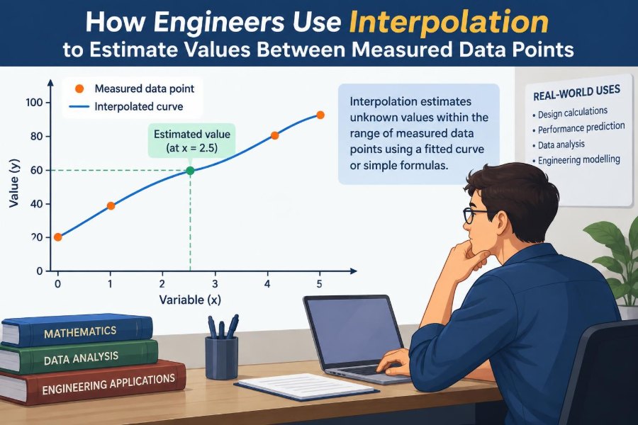
Interpolation fills an internal gap in that measured range. If values are known at two or more nearby inputs, it constructs an estimate for an input that lies between them.
It does not create a new measurement. Rather, it uses a model of how the data behave locally, ranging from a straight line to a smooth curve.
📍 Interpolation Versus Extrapolation
The boundary matters. Interpolation estimates inside the range covered by observations. Extrapolation estimates beyond the first or last observation.
Suppose a pump curve has measurements between 20 and 80 L/s. Estimating head at 50 L/s is interpolation. Predicting head at 100 L/s is extrapolation, where the actual curve may bend, flatten, or enter an operating regime not represented by the data.
Extrapolation is not automatically wrong, but it needs stronger physical justification. Interpolation is generally less risky because it is anchored by data on both sides of the estimate.
🧱 The Coordinates Behind Every Data Set
Interpolation starts with pairs of values, often written as (x, y). The x-value is the independent variable, such as time or temperature, and y is the measured response, such as force or resistance.
For two points, engineers write (x0, y0) and (x1, y1). The task is to estimate y at some target x between x0 and x1.
Before calculation, check that the units are consistent and the independent variable is correctly ordered. A surprisingly large share of spreadsheet mistakes comes from mixing minutes and seconds, Celsius and Kelvin, or unsorted timestamps.
📐 Linear Interpolation: The Default Starting Point
Linear interpolation assumes the response changes at a constant rate between two adjacent measurements. Graphically, it draws a straight line through the two points and reads the value on that line.
The formula is:
y = y0 + (x - x0) × (y1 - y0) / (x1 - x0)The fraction (x − x0) / (x1 − x0) tells us how far the target lies across the interval. That same fraction of the total change in y is added to the first measured value.
🔢 A Worked Pressure Example
Return to the pressure readings: 420 kPa at 10:00 and 460 kPa at 10:10. At 10:06, the target is six tenths of the way through the ten-minute interval.
Pressure = 420 + (6 / 10) × (460 - 420)
         = 420 + 24
         = 444 kPa
The estimated pressure is 444 kPa if a straight-line change is a reasonable local approximation. It is not proof that pressure truly rose uniformly; it is an explicit and reproducible estimate based on the available readings.
⚖️ Interpolation as a Weighted Average
Linear interpolation can also be viewed as a weighted average. A point near the lower measurement should be influenced more strongly by it; a point near the upper measurement should lean more heavily on the upper value.
For a fraction t across the interval, where t runs from 0 to 1, the estimate is:
y = (1 - t)y0 + ty1At the midpoint, t = 0.5, so each endpoint receives equal weight. This viewpoint is useful in computer graphics, finite-element post-processing, and any calculation that blends values between nodes.
🕰️ Estimating Signals Between Sample Times
Data acquisition systems sample continuously changing signals at discrete times. Engineers often interpolate when two instruments have different sample clocks or when a calculated event falls between recordings.
For slowly changing temperature, tank level, or battery state, linear interpolation may be adequate at a suitable sampling interval. For vibration, switching signals, impact loads, or fast control loops, a straight line between sparse samples can hide important peaks and oscillations.
The sampling process itself sets a limit: information not captured by the instrument cannot be reliably reconstructed just by choosing a more elaborate interpolation formula.
🌡️ Reading Calibration Tables
Calibration tables connect an instrument output to a physical quantity. A thermistor table, for example, may list resistance at selected temperatures; a flow meter may list output current at reference flow rates.
If a measured input falls between two tabulated entries, interpolation converts it into an estimated engineering value. This is often more practical than deriving a complete physical equation for every sensor.
Use the table’s stated conditions. A calibration made for one pressure, fluid, supply voltage, or installation arrangement may not apply unchanged under another condition.
🗺️ Estimating Values Across Space
Interpolation is not limited to time. Surveyed elevations, soil properties, air measurements, and measured deflections all vary with position.
Along a single line, the same one-dimensional methods apply. Between points on a surface, engineers may need interpolation in two dimensions, using nearby grid points or mesh nodes.
A contour map is a familiar visual example: its contour lines represent estimated locations of equal elevation between surveyed points. Their reliability depends on point density and terrain complexity.
🧩 Bilinear Interpolation on a Grid
When values are known at the four corners of a rectangular grid cell, bilinear interpolation estimates a value inside it. It first interpolates in one direction along two opposite edges, then interpolates between those two intermediate results.
This method appears in lookup tables for engine control, thermal-property tables, digital terrain models, and image resampling. It is straightforward and continuous across a well-organized grid.
It assumes the variation within that cell can be reasonably represented by blended straight-line changes. A sharp boundary inside the cell, such as a material interface, can make that assumption poor.
🔺 Interpolation on Engineering Meshes
Finite-element analysis divides a component or structure into small elements. The solver computes primary values at nodes, then uses element shape functions to estimate displacement, temperature, stress-related quantities, or other fields within an element.
For a simple triangular element, interpolation is often based on the point’s relative position within the triangle. The nodal values are weighted so that the estimate exactly matches each value at its own node.
This does not mean every displayed contour is equally accurate. Mesh density, element quality, material modeling, boundary conditions, and the quantity being plotted all affect confidence in the result.
📈 When Curvature Makes a Straight Line Weak
Linear interpolation is most defensible over a short interval where the response is nearly straight. It becomes less suitable when the underlying relationship visibly curves or changes rapidly.
For example, the volume of a horizontal cylindrical tank does not vary linearly with liquid depth. Near the bottom and top, a small depth change can correspond to a different volume change than it does near the middle.
More measurements reduce the interval length, often improving a piecewise linear estimate without forcing a single complex curve over the entire data set.
🌊 Polynomial Interpolation and Its Appeal
Polynomial interpolation fits a polynomial through several data points. A quadratic can pass through three points, while higher-degree polynomials can pass through more.
This can represent gentle curvature efficiently and is useful in carefully controlled numerical procedures. However, a polynomial that matches every input point exactly is not automatically a better representation of the physical system.
With many points, one high-degree polynomial may oscillate between data values, especially near the edges of the interval. It can be mathematically exact at the samples and physically implausible between them.
🪢 Splines: Smooth Curves Built in Pieces
A spline uses low-degree polynomials over small adjacent intervals rather than one polynomial across the whole range. The pieces are joined so the curve, and often its slope, changes smoothly.
Cubic splines are common when a smooth estimate is needed for motion paths, tabulated material properties, or signal processing. They can look more realistic than piecewise straight segments when the underlying response is genuinely smooth.
Smoothness is not a substitute for evidence. A spline can overshoot between points, creating values above or below all nearby measurements. This is problematic for quantities that should remain nonnegative or monotonic.
📉 Shape-Preserving Methods for Constrained Data
Some engineering data have known shape constraints. Cumulative mass should not decrease with time; many calibration curves should remain monotonic; a bounded fraction should stay between zero and one.
Shape-preserving interpolation methods are designed to avoid artificial wiggles and overshoot. They may be less visually smooth than a standard cubic spline, but they can better respect the behavior required by the application.
Choose the constraint because the physics or definition supports it, not because a graph seems nicer. Real measurements can decrease due to noise, drift, or a genuine process change.
🧪 Interpolating Experimental Results
Laboratory tests often provide a measured curve rather than a closed-form equation. Engineers interpolate to read values such as stress at a specified strain, torque at a selected speed, or concentration at a chosen time.
First inspect the raw data and test conditions. A missing point near a yield transition, phase change, slip event, or instability may be much less safely estimated than a point within a calm, repeatable region.
Replicate tests can reveal scatter. Interpolating a single noisy run may be appropriate for that specimen, but it should not be casually presented as a universal material property.
🔍 Measurement Noise Changes the Question
Interpolation assumes the listed points are useful anchors. In reality, measurements include noise, resolution limits, offsets, and possible outliers.
An exact interpolating curve passes through every observed point, including random fluctuations. If the goal is to estimate the underlying trend rather than reproduce each noisy reading, fitting or smoothing may be more appropriate.
This distinction is crucial: interpolation honors the data points; regression estimates a broader relationship. Neither is inherently superior; they answer different questions.
📊 Interpolation, Regression, and Curve Fitting
Regression chooses model parameters that make a curve reasonably close to many measurements, usually without requiring it to pass through every one. It is often used where noise is expected and a physical or empirical relationship is needed.
Interpolation is often preferred for a trusted calibration table or numerical solution where the tabulated points must be retained exactly. Regression may be preferable for noisy test data, forecasting, or finding a compact approximate model.
| Approach | Primary purpose | Does it pass through every data point? |
|---|---|---|
| Interpolation | Estimate between known observations | Usually yes |
| Regression | Estimate an overall trend or relationship | Usually no |
| Extrapolation | Estimate outside observed range | Not applicable |
🧠 Let Physics Guide the Method
Data alone do not always identify the right interpolation. Physical understanding provides valuable guardrails.
If a quantity must be positive, conserve mass, remain below a known limit, or follow a known constitutive relation, the chosen procedure should be checked against those facts. A mathematically smooth curve that violates a physical constraint deserves scrutiny.
Sometimes the best approach is to transform the data or interpolate a physically meaningful variable instead. For quantities varying approximately exponentially, interpolation on a logarithmic scale may better reflect the mechanism, provided all values and units are suitable for that transformation.
📏 Data Spacing Controls Local Confidence
Close measurements usually support more credible local estimates than widely separated ones, assuming comparable data quality. A short interval gives less room for unobserved curvature or events.
Uniform spacing is convenient but not always efficient. Engineers often collect points more densely where a response changes quickly, has a threshold, or is particularly consequential, and less densely in stable regions.
A dense collection of poor measurements is not automatically valuable. Calibration, repeatability, sensor placement, and relevant operating conditions matter as much as the number of entries.
🚧 Discontinuities Cannot Be Smoothed Away
Some systems have abrupt changes: a relay switches, a valve opens, a crack forms, a material changes phase, or a control logic branch changes state. Interpolation across that event can produce values that never physically occurred.
For example, averaging data immediately before and after an on/off switch transition may imply a partially on state that does not exist. Treat the regions separately, locate the transition more accurately if necessary, or use a model that represents the discontinuity.
Plotting the data is often the quickest way to notice this risk.
🧮 Units, Rounding, and Significant Digits
Interpolation cannot justify more precision than the inputs provide. If readings are recorded to the nearest whole kilopascal, reporting an interpolated value as 444.372 kPa suggests false certainty.
Carry extra digits during internal calculations to avoid avoidable rounding error, then report a result consistent with instrument resolution and decision needs. The appropriate rounding may differ between an exploratory plot and a manufacturing acceptance limit.
Also avoid interpolating directly between values expressed on incompatible scales without converting first. Temperature differences in Celsius and Kelvin are equivalent, but absolute-temperature relations and logarithmic units require particular care.
💻 Spreadsheet Implementation Without Hidden Errors
For small tables, a spreadsheet formula is often enough. Identify the two rows that bracket the target value, then apply the linear formula with cell references.
Build checks into the sheet:
- Confirm that the target lies within the selected interval.
- Flag duplicate independent-variable values, which would cause division by zero.
- Keep units in column headings rather than relying on memory.
- Test that entering an exact table input returns the corresponding table output.
- Plot the data and interpolated result when the decision is consequential.
For large data sets, lookup functions or scripts can locate bracketing values automatically. Their convenience does not remove the need to inspect edge cases and missing data.
🧑💻 A Simple Algorithm for Tabulated Data
A robust one-dimensional workflow is uncomplicated. Sort the table by the independent variable, find neighboring values that surround the target, and calculate using those neighbors.
- Validate that the target is inside the approved data range.
- Find xi ≤ x ≤ xi+1.
- Check that the interval is nonzero and both corresponding values are valid.
- Apply the selected interpolation rule.
- Return the result with a status or warning if the target is at a boundary or data quality is questionable.
Production software should define what happens at missing values, repeated inputs, out-of-range requests, and discontinuity markers. Silent fallback to extrapolation is a poor default for safety-relevant calculations.
🛠️ Choosing a Method for the Job
Method selection should match the data, physics, and consequence of error. The most sophisticated curve is not necessarily the safest or clearest choice.
| Situation | Often suitable starting point | Main caution |
|---|---|---|
| Two nearby, slowly varying readings | Linear interpolation | Check for unobserved curvature |
| Regular two-variable lookup table | Bilinear interpolation | Check behavior at cell boundaries |
| Smooth, reliable tabulated curve | Spline or low-order local method | Watch for overshoot |
| Monotonic calibration data | Shape-preserving method | Verify monotonicity is physically justified |
| Noisy experimental observations | Regression or smoothing, then estimate | Do not mistake the fit for raw measurement |
⚠️ Common Misuses of Interpolation
One common error is using distant points simply because they are available. Another is treating an interpolated result as an independently verified reading.
Other traps include fitting high-order curves to sparse data, bridging a discontinuity, overlooking an outlier, and applying a calibration outside its specified conditions. Each can produce a precise-looking number with weak engineering meaning.
When the result influences a design limit, alarm threshold, or safety decision, document the source data, method, interval, assumptions, and any expected uncertainty.
✅ A Practical Quality Check
Before relying on an interpolated value, ask a small set of direct questions:
- Is the target truly between relevant measured points?
- Are the measurements trustworthy and taken under comparable conditions?
- Is the response expected to be smooth over this interval?
- Does the estimate respect known physical limits and units?
- Would a plausible error in the estimate change the decision?
If the last answer is yes, collect another measurement, reduce the interval, use an independently justified model, or perform a sensitivity check. The right response to uncertainty is not always a more complicated equation.
🧰 Interpolation in Everyday Engineering Work
Interpolation often operates quietly inside engineering tools: reading property tables, synchronizing test channels, displaying simulation contours, converting sensor output, and estimating a value at a design operating point.
Its value lies in making incomplete measurements usable without pretending they are complete. A transparent local estimate can be more defensible than an elaborate black-box prediction.
It also helps communication. When a report states that a value was linearly interpolated between specified readings, another engineer can inspect, reproduce, and challenge the assumption if needed.
🎯 The Core Principle: Estimate Locally, Think Critically
Interpolation is fundamentally an act of informed approximation. It works best when nearby data represent the same physical regime, the chosen curve reflects plausible behavior, and the requested point remains within the data range.
Linear interpolation is a powerful baseline because it is transparent, stable, and easy to audit. Curved, multidimensional, shape-preserving, and physics-aware methods extend the idea when the situation calls for them.
The essential discipline is to separate what was measured from what was estimated. That distinction keeps calculations useful without giving them more authority than the data can support.
Good interpolation turns measured points into practical engineering insight by making assumptions visible, local, and testable. Used with sound judgment, it bridges gaps in data without hiding the limits of what is known. 📏📊🔧