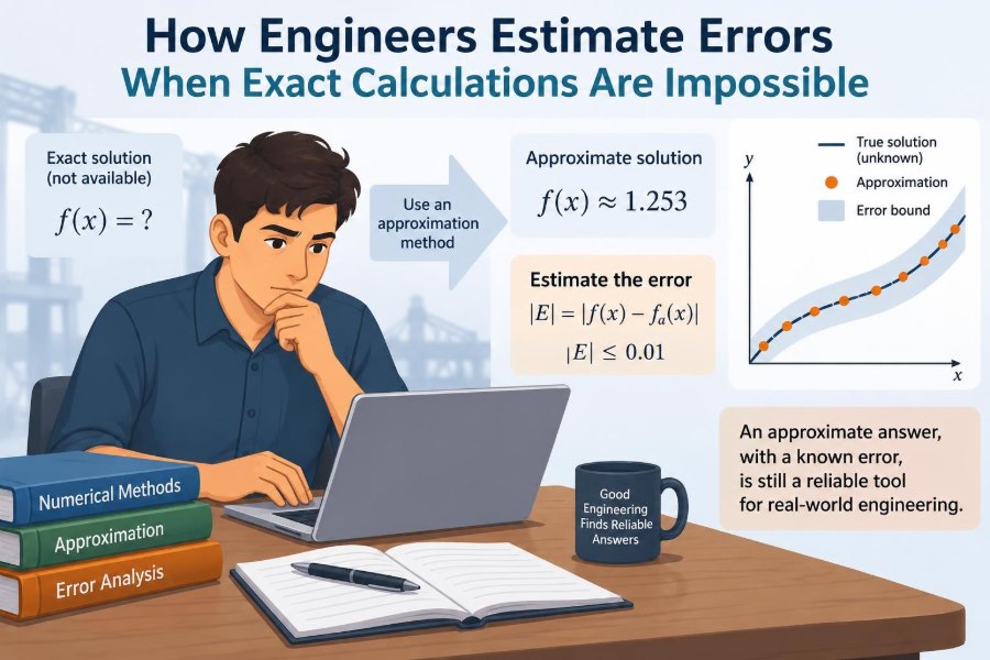

A bridge is designed using dimensions measured on site, material properties measured in a laboratory, and loads estimated from expected use. None of those inputs is perfectly exact. Yet the bridge still has to be safe, economical, and buildable.
The same problem appears at smaller scales. A machinist checks a shaft diameter with a micrometer. A controls engineer reads a noisy temperature sensor. A civil engineer predicts rainfall runoff from an incomplete record. Real decisions cannot wait for perfect information.
Engineering mathematics provides ways to ask a more useful question than “Is this answer exact?” The better question is: how far could this answer reasonably be from the truth, and does that uncertainty change the decision?
Error estimation turns imperfect measurements and simplified models into decisions that can be checked, communicated, and improved. It is not an admission of failure; it is part of professional engineering judgment.
🎯 Exact Answers Are Rare in Engineering
An exact calculation assumes exact inputs and a perfectly faithful mathematical model. Both conditions are unusual outside carefully controlled problems.
Measurements have limited resolution, physical systems vary, and models omit details that are too small, uncertain, or expensive to include. Engineers therefore work with estimates accompanied by a stated level of confidence or bound.
This distinction matters because a calculator can display many digits even when only the first few are meaningful. More displayed digits do not create more knowledge.
🧭 Error Is a Difference, Not a Blunder
In engineering, error usually means the difference between an estimated value and a reference value. It does not automatically mean someone made a mistake.
If a measured length is 10.02 mm and the accepted reference is 10.00 mm, the signed error is 0.02 mm. The sign tells direction: positive means the estimate is high relative to the reference; negative means it is low.
Often the reference value is unknown. In that situation, engineers cannot calculate the actual error directly. They estimate an uncertainty: a credible range describing what the true value may be.
📏 Absolute, Relative, and Percentage Error
Three related quantities help put deviations in context. Absolute error is the magnitude of the difference, written as |estimated − reference|.
Relative error divides that difference by the reference value. Percentage error multiplies the relative error by 100. A 0.1 mm discrepancy means something very different for a 1 mm feature than for a 10 m beam.
| Measure | Useful question | Example use |
|---|---|---|
| Absolute error | How large is the difference in physical units? | Checking a 0.02 mm machining deviation |
| Relative error | How large is it compared with the quantity? | Comparing errors across component sizes |
| Percentage error | How easily can the relative error be communicated? | Reporting an estimate to a non-specialist audience |
Percentage error can mislead when the reference value is close to zero, because division by a tiny number makes the percentage enormous. In such cases, absolute error is usually more informative.
🔍 Accuracy and Precision Describe Different Things
Accuracy means closeness to the true or accepted value. Precision means repeatability: whether repeated readings cluster closely together.
A scale that reads consistently 0.5 kg too high is precise but inaccurate. A scale that gives scattered readings around the true value may be accurate on average but imprecise for a single measurement.
Engineers need both ideas. Calibration primarily addresses accuracy, while improved instruments, stable procedures, and repeated observations can improve precision.
🎲 Random Error Creates Scatter
Random error changes unpredictably from one observation to another. Electrical noise, small reading variations, vibration, and changing environmental conditions can all cause it.
Suppose a technician measures a voltage several times and obtains slightly different values. If the measurement process has no strong directional bias, the readings may scatter around the true value.
Repeated measurements can reduce the influence of random variation on an average. They do not guarantee perfection, but averaging is often more reliable than relying on one reading.
⚠️ Systematic Error Shifts Every Result
Systematic error pushes results consistently in one direction. A sensor with a zero offset, a stretched tape measure, or an incorrect conversion factor can produce this pattern.
Taking more measurements does not remove a systematic error. Averaging a hundred readings from a biased sensor simply produces a highly repeatable biased answer.
This is why calibration against a known reference, independent checks, and careful review of assumptions are essential. Random scatter is visible in repeated readings; systematic bias can hide behind apparently tidy data.
🧰 Instrument Resolution Sets a Basic Limit
No instrument can report detail smaller than its useful resolution. A ruler marked every millimetre cannot justify a length reported to four decimal places in millimetres.
A common practical estimate is that manual reading uncertainty is some fraction of the smallest division, depending on the instrument and method. Digital instruments have display resolution too, but their real uncertainty may be larger because of calibration, noise, or sensor response.
Resolution is therefore a starting point, not a complete uncertainty statement.
🌡️ The Measurement Environment Also Matters
Temperature, humidity, vibration, electromagnetic interference, alignment, and operator technique can influence a measurement. These effects are especially relevant when tolerances are tight.
For example, a metal part changes size slightly with temperature. Measuring it immediately after machining, while it is warmer than the inspection environment, can create a meaningful difference for precision work.
The practical response is not to control every variable blindly. It is to identify variables capable of changing the decision and either control, measure, or include them in the uncertainty estimate.
🧮 Rounding Introduces Its Own Error
Rounding replaces a value with a nearby representable number. If 3.14159 is rounded to 3.14, the rounding error is small for many purposes but not for every calculation.
Repeated intermediate rounding can accumulate or distort results, particularly when calculations subtract nearly equal numbers. Keep sensible internal precision and round only when reporting a final result.
Reported digits should match the uncertainty. Writing 12.347891 N suggests a degree of knowledge that may not exist if the load is only known within a few tenths of a newton.
💻 Numerical Methods Trade Exact Formulas for Approximations
Many engineering equations cannot be solved conveniently in closed form. Numerical methods approximate the answer through repeated arithmetic steps.
Finite differences approximate derivatives, numerical integration approximates areas, and iterative solvers approximate roots of equations. The approximation depends on settings such as step size, mesh density, or stopping tolerance.
The numerical result can look stable while still being wrong if the model, setup, or algorithm is unsuitable. A solver output is evidence, not an automatic certificate of truth.
📉 Truncation Error Comes from Stopping Early
Truncation error occurs when an infinite or exact mathematical process is cut off. Approximating a curved response with a few terms of a series, or a derivative with a finite difference, leaves out remaining terms.
Smaller numerical steps often reduce truncation error, but only up to a point. Very small steps can magnify round-off effects in computer arithmetic or make computation unnecessarily expensive.
Good numerical work balances competing errors rather than assuming “smaller” is always “better.”
🧱 Discretisation Replaces a Continuum with Pieces
Finite element and finite volume models divide a continuous object or field into elements, cells, or nodes. This is called discretisation.
A coarse mesh may miss a sharp stress concentration near a hole or a steep temperature gradient near a heat source. A finer mesh can capture more detail, but it also requires more computing time and careful model setup.
Mesh refinement is a practical test: if a key result changes significantly as the mesh is refined, the original mesh was not yet adequate for that result.
🔁 Iterative Solvers Need a Stopping Rule
Many calculations improve an initial guess repeatedly until a residual becomes small. A residual measures how well the current estimate satisfies the governing equations.
A small residual is useful, but it is not the same as a small real-world error. An iterative solver can solve the wrong model extremely well.
Choose tolerances based on the required decision accuracy, scale variables appropriately, and check whether further iterations materially change quantities that matter, such as peak stress or pressure drop.
📐 Linearisation Makes Difficult Relationships Manageable
Linearisation approximates a curved function by a straight line near an operating point. It is the mathematical reason small input changes can often be translated into estimated output changes.
For a function y = f(x), a small change Δx gives an approximate output change Δy ≈ f′(x)Δx. The derivative f′(x) describes local sensitivity.
This works best when changes are small and the function is smooth over the relevant range. It becomes unreliable near sharp nonlinear behaviour, discontinuities, saturation, or thresholds.
📦 Propagating Uncertainty Through a Formula
Inputs do not stay uncertain in isolation. When they enter a calculation, their uncertainties affect the output. This is called uncertainty propagation.
Consider the area of a rectangle, A = LW. If length and width each have some uncertainty, the calculated area has uncertainty too. For small independent relative uncertainties, a useful worst-case approximation is that the relative area uncertainty is roughly the sum of the relative uncertainties in L and W.
This approximation is conservative when all errors could align in the most unfavorable direction. It is often suitable for early design checks, but its assumptions should be stated.
➕ Combining Independent Random Uncertainties
When uncertainty sources are independent and behave like random variations, engineers often combine them by root-sum-square rather than adding every maximum directly.
If quantities have standard uncertainties u1, u2, and so on, a combined estimate is often represented by the square root of u12 + u22 + … . This prevents an unrealistically pessimistic total when independent variations are unlikely to peak together.
The method is not a universal shortcut. It depends on how uncertainty is defined, whether distributions are reasonable, and whether inputs truly are independent.
🔗 Correlation Can Defeat Simple Combination Rules
Two inputs are correlated when they tend to vary together. For example, two dimensions measured with the same miscalibrated instrument may share a common offset.
Ignoring correlation can understate or overstate uncertainty. If two errors move in the same direction, their effects may reinforce each other; if they move oppositely, they may partly cancel.
Whenever multiple values share equipment, a common environment, a common data source, or a common model assumption, independence should be questioned rather than assumed.
📊 Sensitivity Analysis Finds What Deserves Attention
Sensitivity analysis asks how much an output changes when each input changes. It directs effort toward the assumptions and measurements that actually control the result.
For a pump-system model, changing pipe roughness may barely affect predicted flow while changing valve position affects it strongly. Improving the roughness estimate first would offer little practical return.
A simple approach is to vary one input at a time over a credible range and observe the output change. More advanced approaches vary several inputs together, which is useful when interactions are important.
🕳️ Worst-Case Bounds Serve Safety-Critical Decisions
A worst-case calculation assumes uncertainties take values that produce the most adverse credible outcome. This can be appropriate when failure consequences are severe or when data are sparse.
The drawback is conservatism. Combining every extreme simultaneously can produce a scenario that is mathematically possible but physically very unlikely, leading to unnecessary cost or weight.
Engineers therefore distinguish between a conservative design bound and a realistic operating prediction. Both can be useful, but they answer different questions.
🎯 Probabilistic Estimates Describe Likely Variation
Probabilistic methods model uncertain quantities as distributions rather than single bounds. They can estimate how output variation follows from input variation.
Monte Carlo simulation is a common approach: sample plausible input values many times, run the model repeatedly, and inspect the resulting outputs. It is particularly helpful for nonlinear models where simple propagation formulas become weak.
Its output is only as credible as its inputs. Assigning a neat distribution without adequate measurement, physical reasoning, or expert review can create false confidence.
🧪 Model Error Is Not Measurement Error
A model can use perfectly measured inputs and still be wrong because it omits relevant physics or uses an inappropriate approximation. This is model-form error.
For instance, treating a complex flow as steady and uniform may be useful for an early estimate but inadequate near rapid transients or complex geometry. The issue is not arithmetic; it is whether the model represents the decision-relevant behaviour.
Validation compares model predictions with independent observations where possible. Agreement under one condition does not automatically validate the model under every operating condition.
🧩 Verification Checks the Mathematics and Code
Verification asks, “Did we solve the equations correctly?” Validation asks, “Are these the right equations for reality?” Both are needed.
Useful verification checks include comparing against a hand calculation, testing a simplified case with a known solution, checking units, refining a mesh, or changing a time step. These checks can reveal implementation and numerical errors before results are trusted.
A sophisticated simulation without verification is still vulnerable to simple mistakes such as a sign error, an incorrect boundary condition, or inconsistent units.
🧾 Units Are an Error-Detection Tool
Dimensional analysis checks whether units are consistent through an equation. If one side of an energy equation is in joules and the other is in newtons, something is wrong.
Unit checks do not prove the physics is correct, but they catch many common failures: mixing millimetres and metres, confusing mass with force, or applying an empirical formula outside its intended unit system.
Make units visible in calculations, data files, plots, and reports. Hidden unit conversions are a frequent source of avoidable engineering error.
🧠 Significant Figures Communicate Credible Precision
Significant figures are a communication discipline, not a substitute for an uncertainty analysis. They prevent a result from claiming detail unsupported by measurements or modelling.
If a calculated deflection is 4.236 mm but the inputs and model support only about a tenth of a millimetre, reporting 4.2 mm may be more honest. In some contexts, reporting 4.2 ± 0.1 mm is better still.
Keep extra digits during calculation when needed, then round deliberately at the point of communication.
🗂️ An Uncertainty Budget Makes Assumptions Visible
An uncertainty budget is a structured list of significant uncertainty sources, their estimated size, and how they affect the final result. It transforms a vague statement such as “there may be error” into a reviewable argument.
A useful budget may include instrument calibration, repeatability, environmental effects, geometry assumptions, material-property variation, numerical settings, and model limitations. Not every source needs equal detail.
The goal is prioritisation. If one source dominates, improving minor sources will not materially improve the answer.
🛠️ A Practical Workflow for Estimating Error
- Define the decision and the output quantity that matters.
- List measured inputs, assumed inputs, and model choices.
- Identify likely uncertainty sources for each.
- Estimate their size using calibration information, repeat measurements, physical bounds, or justified engineering assumptions.
- Propagate the important uncertainties through the calculation.
- Check sensitivity, numerical convergence, units, and plausibility.
- Report the result with its limits and explain what would change the conclusion.
This workflow scales from a spreadsheet calculation to a major simulation study because it focuses on traceable reasoning rather than a particular software package.
🚫 Common Ways Error Estimates Go Wrong
- Confusing precision with accuracy: tightly clustered readings can still be biased.
- Adding every uncertainty blindly: this may be needlessly conservative or statistically unjustified.
- Ignoring shared causes: correlated inputs cannot always be treated as independent.
- Using a fine numerical model without convergence checks: more elements alone do not guarantee a trustworthy result.
- Reporting a single number without conditions: readers need to know the assumptions behind it.
Most of these failures are prevented by writing assumptions down early and inviting review before the calculation becomes elaborate.
🗣️ Communicating Uncertainty Supports Better Decisions
An error estimate should be understandable to the person making the decision. “Predicted peak temperature is 82 °C under the stated operating assumptions, with the result most sensitive to heat-transfer coefficient” is more useful than a bare number.
State whether a range is a worst-case bound, an estimated measurement uncertainty, or a probabilistic interval. These descriptions are not interchangeable.
Clear uncertainty communication helps teams decide whether to test further, increase a safety margin, redesign a component, or proceed because the uncertainty does not affect the decision.
✅ The Core Principle: Make Uncertainty Useful
Exact calculation is often impossible because engineering starts with imperfect observations and simplified representations of reality. The solution is not to hide that imperfection behind extra decimal places.
Estimate the dominant sources of uncertainty, understand how they move through the model, test whether the result is numerically stable, and connect the remaining uncertainty to the decision at hand.
Good engineering is not the search for a magically exact number. It is the disciplined practice of knowing what a number means, where it can fail, and whether it is reliable enough for its intended use.
Engineers make sound decisions not by eliminating every error, but by identifying, bounding, and managing the errors that matter. 📉📐🔧