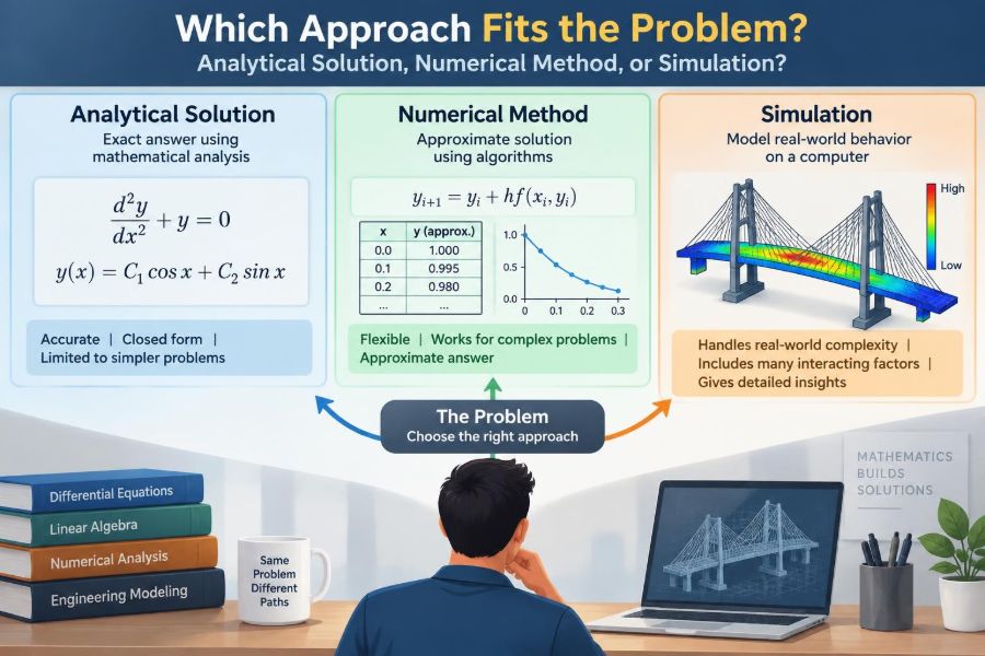

A structural engineer needs the deflection of a beam. A process engineer needs to predict heat loss from a reactor. A designer wants to know whether a drone will remain stable in gusty wind. Each problem involves mathematics, but the best route to an answer is not automatically the same.
Sometimes a compact equation gives an exact result and exposes the physics beautifully. Sometimes the governing equation is known but cannot be rearranged into a useful formula, so a numerical algorithm is the practical choice. And sometimes the system is so interconnected, uncertain, or dynamic that a simulation is needed to observe possible behavior over time.
Choosing poorly can waste computation, hide an error behind impressive graphics, or produce a neat formula that does not represent the real situation. Choosing well helps engineers make decisions with an appropriate balance of speed, accuracy, insight, and cost.
The useful question is not “Which method is best?” It is: which approach gives an answer reliable enough for this decision, given the model, data, time, and uncertainty available?
🧭 Start with the Decision, Not the Tool
Before selecting software or writing equations, identify the decision the analysis must support. Is the aim to size a component, understand a trend, compare design alternatives, diagnose a failure, or estimate a safety margin?
A preliminary concept may only require an order-of-magnitude estimate. A final design check for a heavily loaded component may require a higher-fidelity model, careful verification, and documented assumptions. The required answer determines the appropriate method.
📘 What an Analytical Solution Means
An analytical solution is an explicit mathematical expression derived from governing equations and assumptions. For example, a falling object in a vacuum follows a position formula obtained directly by integrating constant acceleration.
Analytical does not merely mean “done by hand.” Symbolic algebra software can derive or manipulate analytical expressions. The defining feature is that the result is expressed as a formula or exact mathematical relationship rather than as values calculated step by step at discrete points.
🔢 What a Numerical Method Means
A numerical method obtains an approximate answer through arithmetic operations and an algorithm. It may solve an equation, integrate a function, or approximate a differential equation at a finite set of points.
Newton’s method for finding roots, numerical quadrature for areas, and finite-difference methods for temperature fields are all numerical methods. Their answers are usually arrays, tables, or computed values rather than a single general formula.
🎬 What Engineering Simulation Means
A simulation is a computational representation of a system that is run under specified conditions. It often uses numerical methods internally, but simulation is broader: it includes the model structure, inputs, operating rules, events, time progression, and interpretation of output.
For example, a traffic simulation may track individual vehicles, signals, lane changes, and random arrivals. Its numerical calculations matter, yet the central purpose is to imitate system behavior under scenarios that are difficult to observe or test directly.
🧩 The Three Approaches Overlap
These categories are useful, but they are not competing boxes. A simulation may contain an analytical formula for motor torque, numerical integration for vehicle motion, and empirical data for tire behavior.
Likewise, engineers often begin with an analytical estimate, use a numerical model to refine it, and then simulate realistic operating scenarios. The strongest workflow is often a layered one, not a single-method choice.
🗺️ A Quick Comparison
| Approach | Typical output | Best suited to | Primary limitation |
|---|---|---|---|
| Analytical solution | Formula, closed-form relationship | Simple geometry, idealized conditions, insight | Requires restrictive assumptions |
| Numerical method | Approximate values or fields | Known equations with complex shapes or conditions | Discretization and convergence errors |
| Simulation | Scenario behavior, time histories, distributions | Interacting, dynamic, uncertain systems | Model complexity can obscure weak assumptions |
The table is a starting point, not a rulebook. A simple simulation can be less reliable than a carefully checked numerical calculation, while a well-designed numerical model can be more useful than an elegant analytical expression built on unrealistic assumptions.
⚙️ Begin with the Governing Physics
Ask what principles control the system: conservation of mass, momentum, energy, electric charge, or another physical law. If the governing relationship is uncertain, no amount of computation can fully compensate for that uncertainty.
For a pipe-flow problem, pressure loss may depend on flow rate, diameter, roughness, fluid properties, fittings, and flow regime. The first challenge is deciding which effects matter enough to include, not deciding whether to press “run.”
🧱 When Assumptions Make an Analytical Model Possible
Analytical solutions usually become possible when the model has regular geometry, simple boundary conditions, and linear or separable equations. A uniform beam, a one-dimensional steady heat path, or an ideal electrical circuit often fits this pattern.
These assumptions are not automatically flaws. They are deliberate simplifications. The key question is whether leaving out an effect changes the decision. Neglecting air resistance may be acceptable for a short laboratory demonstration but poor for predicting the terminal speed of a parachute.
✨ Why Analytical Results Are So Valuable
A formula shows how variables relate. If beam deflection is proportional to load and inversely related to stiffness, the engineer immediately sees which design changes have the greatest leverage.
Analytical results are also fast to evaluate, easy to differentiate, and useful for checking units and limiting behavior. They make excellent first estimates and provide reference cases for validating numerical code.
🚧 Where Closed-Form Solutions Stop Helping
Real systems often involve irregular geometry, nonlinear material behavior, changing contact conditions, turbulence, chemical reactions, or mixed boundary conditions. The governing equations may still be known, but a manageable explicit formula may not exist.
Forcing such a system into a simple formula can create false confidence. A result is not more trustworthy merely because it is written compactly on one line.
🧮 Discretization: Turning Continuity into Computation
Numerical methods commonly divide a continuous problem into finite pieces. A beam becomes nodes and elements; a heat-transfer domain becomes a grid; time becomes a sequence of increments.
This process is called discretization. It replaces an infinite set of possible locations or times with a finite set that a computer can evaluate. The approximation is controlled by mesh size, time step, interpolation choices, and the selected numerical scheme.
📈 Root Finding for Design Calculations
Many engineering questions reduce to finding a value that makes an equation equal zero. Suppose a pump curve and a piping-system curve are expressed as functions of flow rate. Their operating point occurs where the difference between them is zero.
Numerical root-finding methods can locate that point even if the equation cannot be rearranged neatly. A robust method such as bisection is slower but dependable when a sign-changing interval is known; faster methods may need a good starting guess and can fail when the function behaves unexpectedly.
🌡️ Numerical Integration and Differential Equations
Some quantities are accumulated effects: energy transferred over time, distance from changing velocity, or total load from a distributed pressure. Numerical integration approximates these quantities by summing many small contributions.
Differential equations add another layer because they describe rates of change. A numerical solver advances the system from one state to the next. Its time step must be small enough to capture relevant changes without making the computation unnecessarily expensive.
🕸️ Finite Elements and Finite Differences
Finite-difference methods approximate derivatives using nearby grid values. They are especially natural on simple, structured domains such as a rectangular plate or a one-dimensional pipe.
The finite element method divides a domain into small connected elements and approximates the unknown field within each element. It is widely used because complex component shapes, material regions, and support conditions can be represented more flexibly.
Neither method is simply “more accurate.” Accuracy depends on the equation, geometry, element or grid quality, boundary conditions, and verification process.
⏱️ Steady-State and Transient Questions
A steady-state model asks what the system looks like after conditions have settled. A transient model asks how it changes with time. A wall’s final temperature distribution may be steady; the warm-up of that wall is transient.
Use transient analysis only when timing matters. Starting currents, vibration response, thermal cycling, control actions, and emergency shutdowns often require it. For a genuinely settled operating condition, a transient simulation can add effort without adding decision value.
🎲 Why Simulation Becomes Necessary
Simulation is particularly useful when many rules and interactions shape the outcome. Consider a manufacturing line: machine failures, repair delays, buffer sizes, worker schedules, inspection rework, and variable arrivals can interact in ways no single average-rate calculation reveals.
A discrete-event simulation can represent these events as they occur. A computational fluid dynamics simulation can represent evolving flow and heat fields. An agent-based model can represent many individual entities following rules. The right simulation type follows the system behavior.
🌪️ Deterministic and Stochastic Models
A deterministic model produces the same output whenever it receives the same inputs. Many structural, thermal, and circuit calculations are treated this way.
A stochastic model includes randomness, such as variable demand, material scatter, wind fluctuations, or arrival times. One run is then only one possible realization. Engineers often run many trials to examine a range of outcomes rather than treating a single simulated trace as a prediction of exactly what will happen.
🎯 Match Fidelity to the Decision
Model fidelity is the degree to which a model represents relevant features of the real system. More fidelity is not always better. It requires more input data, more computation, more calibration, and more opportunities to make unnoticed setup errors.
If the decision is whether insulation should be approximately 50 mm or 150 mm thick, a one-dimensional heat-loss model may be sufficient. If the decision concerns local condensation near a complex thermal bridge, a detailed spatial model may be justified.
📏 Accuracy Is Not the Same as Precision
A result shown to six decimal places may be numerically precise but physically inaccurate. This happens when the calculation is stable and repeatable while the inputs, assumptions, or model form are wrong.
Keep numerical precision proportionate to input quality. If a load estimate is uncertain or a material property varies meaningfully with temperature, reporting a highly specific final answer can imply knowledge the model does not possess.
🔍 Verification: Did You Solve the Model Correctly?
Verification checks the mathematics and implementation. For numerical work, this can include refining the mesh or time step, checking residuals, comparing methods, testing conservation balances, and recovering known analytical cases.
A mesh-refinement study is a common example. If predicted stress changes substantially whenever the mesh is made finer, the original mesh was not adequate for that quantity. Refinement should continue until the result relevant to the decision is sufficiently stable.
✅ Validation: Is It the Right Model?
Validation asks whether the model represents the real system well enough for its intended use. It compares predictions with appropriate measurements, observed behavior, or trusted benchmark data.
A perfectly verified solver can still be invalid for a particular application. For instance, a heat model may solve conduction accurately but give poor real-world predictions if it omits an important convective airflow path.
🧪 Use Simple Models as Sanity Checks
Even when a detailed simulation is planned, construct a simple estimate first. Calculate an approximate energy balance, limiting load, characteristic time, or expected range. These checks create an independent expectation before complex software produces a polished result.
If a detailed model differs dramatically from the estimate, do not immediately assume the detailed model is superior. Investigate the discrepancy. It may reveal a missing mechanism in the simple model, or an incorrect boundary condition in the detailed one.
🧷 Boundary Conditions Often Control the Answer
Boundary conditions specify how a system interacts with its surroundings: fixed temperature, applied force, electrical potential, flow rate, heat flux, restraint, or contact behavior. They frequently affect results as much as the internal governing equation.
In practice, boundary conditions can be harder to know than material properties. A component described as “fixed” may actually have joint flexibility; an exterior surface may experience changing wind and radiation. Treat uncertain boundaries explicitly rather than hiding them behind convenient defaults.
🧯 Nonlinearity Changes the Method Choice
A system is nonlinear when its response does not scale proportionally with its input. Large deformation, plasticity, contact, friction, radiation, phase change, and many fluid-flow effects introduce nonlinearity.
Nonlinear problems may require iterative numerical solution and can have multiple possible states or sensitivity to starting conditions. Analytical approximations remain useful for understanding, but numerical analysis is often required for credible prediction across the full operating range.
💻 Computational Cost Is an Engineering Constraint
Run time, memory, licensing, hardware access, and analyst time all matter. A model that takes days to run may be unsuitable for rapid design iteration, even if it is theoretically sophisticated.
Cost also includes review. A simpler model can be easier for colleagues to inspect, challenge, maintain, and reuse. For routine decisions, transparent calculations may deliver more organizational value than a complex model understood by only one person.
🧠 Interpretability Has Practical Value
Decision-makers often need to know why a result changes. Analytical models usually make sensitivity visible. Numerical and simulation models can provide the same insight, but it must be extracted deliberately through parameter sweeps, plots, and sensitivity analysis.
When communicating results, distinguish observed model output from causal explanation. A contour plot may show a hot spot; engineering interpretation should explain whether it arises from geometry, low conductivity, inadequate cooling, a boundary condition, or another mechanism.
📊 Sensitivity Analysis Reveals What Deserves Attention
Sensitivity analysis varies selected inputs and observes the resulting change in output. It identifies which uncertainties meaningfully affect the decision and which do not.
For a pressure-drop model, flow rate and pipe diameter may dominate while a minor fitting coefficient has little practical effect. That finding directs effort toward measuring, controlling, or conservatively bounding the inputs that matter most.
⚠️ Common Mistake: Treating Software Output as Evidence
Software produces results, not automatic proof. Color contours, animations, and detailed reports can look authoritative even when the model geometry, material data, contacts, or loading are unsuitable.
Before accepting output, ask: Does the direction of response make physical sense? Are units consistent? Are reactions balanced? Does the result approach a sensible limit? Could the apparent feature be a mesh artifact or numerical instability?
🪤 Common Mistake: Building Detail Before Understanding
Starting with a highly detailed model can lock in assumptions before the problem is framed. It also makes troubleshooting difficult because many possible causes are entangled.
A better sequence is to begin with the simplest model that captures the dominant mechanism. Add detail only when it answers a defined question: Does contact resistance matter? Does transient loading change the peak? Does geometric irregularity create a local concentration?
🔄 A Practical Escalation Workflow
- Define the decision, performance measure, operating conditions, and acceptable uncertainty.
- State the governing physics and make assumptions visible.
- Develop an analytical estimate or dimensional check where possible.
- Select a numerical method if the equations or geometry require approximation.
- Build a simulation when interactions, events, time evolution, or uncertainty distributions are central.
- Verify computation, validate important assumptions, and communicate the range of credible outcomes.
This workflow does not prohibit moving backward. New data may show that a simplification was invalid, while a sensitivity study may show that a detailed feature can be safely removed.
🏗️ Example: Choosing a Method for a Bracket
For a preliminary bracket design, hand calculations based on beam theory can estimate bending stress and deflection. They quickly indicate whether thickness, material, or load path needs to change.
If the bracket has curved cutouts, bolt preload, contact with another component, or local stress concerns, finite element analysis can refine the assessment. A full dynamic simulation is only warranted if time-varying loads, impacts, or vibration behavior drive the design requirement.
🔥 Example: Choosing a Method for Thermal Design
A first calculation for a heated enclosure may use a lumped energy balance: electrical input equals estimated losses through walls and ventilation. This identifies the approximate heater capacity and major loss paths.
A numerical conduction model becomes useful when wall layers, geometry, or localized temperature limits matter. A coupled transient simulation may be justified when control cycling, moving air, product loading, and warm-up time affect performance.
🚦 Example: Choosing a Method for Operations
A simple queueing approximation can help estimate whether a service station is likely to become congested as demand rises. It is useful for early capacity screening.
When arrivals vary by time, service times differ, resources are shared, and failures occur, discrete-event simulation can test scheduling and layout scenarios. The simulation should report distributions and bottlenecks, not just one attractive average waiting time.
📝 Document Assumptions and Limits
A useful engineering result includes its scope. Record material models, loads, boundary conditions, simplifications, solver settings, mesh or time-step checks, input sources, and the conditions under which the conclusion applies.
Documentation is not bureaucracy. It allows another engineer to review the work and allows your future self to understand why the result was credible. It also prevents a result from being reused outside the conditions for which it was developed.
🤝 Communicate the Answer at the Right Level
Technical colleagues may need equations, residual histories, mesh information, and sensitivity results. A project manager may need the design implication, confidence range, main assumptions, and the action required.
Both audiences deserve clarity. Avoid presenting uncertainty as weakness; a clearly stated range and its drivers are often more useful than a single unsupported number.
🏁 The Core Principle: Use the Simplest Credible Model
An analytical solution is ideal when its assumptions preserve the behavior that matters. A numerical method is appropriate when known physics must be solved approximately because of complexity. A simulation is appropriate when the system’s interactions, timing, or uncertainty are themselves part of the question.
The best approach is therefore the one that is simple enough to understand, detailed enough to support the decision, and tested enough to deserve trust. Method choice is an engineering judgment, not a contest between hand calculations and software.
Use equations to understand, numerical methods to resolve complexity, and simulations to explore system behavior—then verify that the answer remains connected to physical reality. 📐🔍⚙️