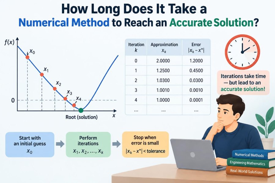

A simulation is running, the residual on the screen is falling, and the iteration counter keeps climbing. You need a result before a design review, a weather forecast deadline, or the next control update. The natural question is simple: how much longer?
Numerical methods turn mathematical models into computable approximations. They solve systems too large, nonlinear, irregular, or time-dependent for an exact formula to be useful. But an approximation is not valuable merely because the software has stopped.
Some methods reach a useful answer in a handful of iterations. Others need thousands. Some appear to converge rapidly and then stall; others give a deceptively small residual while an important engineering quantity is still wrong.
Estimating solution time means understanding both mathematics and computation: what “accurate” means, how quickly error decreases, what each iteration costs, and when the model itself limits the value of further work.
🎯 Start by Defining “Accurate”
A numerical method cannot be said to have reached an accurate solution until there is a target to meet. Accuracy might mean displacement within a specified tolerance, pressure drop correct to enough significant figures, or a control input reliable enough to keep a system stable.
There is no universal tolerance. A preliminary concept study may only need the right order of magnitude. A stress concentration assessment or an orbital trajectory calculation may require a much tighter error bound.
It helps to state the target in terms of the quantity of interest: the specific output that informs a decision. That could be a maximum temperature, total drag, first natural frequency, or probability of failure—not necessarily every value in the computed field.
🧭 Separate the Different Meanings of Error
Several errors can coexist, and reducing one does not automatically reduce the others. A solver’s progress report usually concerns only its own iterative error.
- Model error: the governing equations, material law, boundary conditions, or inputs do not fully represent reality.
- Discretization error: a mesh, time step, or finite approximation replaces a continuous problem.
- Iterative error: an algebraic solver stops before reaching the exact solution of the discretized equations.
- Round-off error: finite-precision arithmetic introduces small numerical limits.
A very small iterative error is worthwhile only when it is not dwarfed by model or discretization error. Spending hours polishing the solution of a coarse mesh is often a poor use of computation.
🔢 Understand What an Iteration Actually Does
An iteration creates an improved estimate from a previous estimate. In a root-finding problem, the estimate may be a single number. In computational fluid dynamics or structural analysis, it may be a vector containing millions of unknown values.
For a linear system written as Ax = b, an iterative method repeatedly updates x so that the equations are increasingly well satisfied. Each update may involve matrix-vector products, preconditioning, communication between processors, and checks for stopping conditions.
The count alone is therefore not a measure of elapsed time. Twenty expensive iterations on a large parallel model can take longer than thousands of cheap scalar iterations.
📉 Convergence Rate Is the First Clock
The main mathematical clue is the convergence rate: the way error shrinks as iterations proceed. If error decreases steadily by a fixed fraction per iteration, the method has linear convergence. If the number of correct digits roughly doubles near the solution, it has quadratic convergence.
In an idealized local form, an error sequence may behave like e_(k+1) ≈ C e_k^p. Here, p describes the order of convergence. Values near 1 indicate linear behavior; values near 2 indicate quadratic behavior.
This relation is most useful once the method is in its expected convergence regime. Early iterations may behave differently, particularly when the initial estimate is poor or the problem is strongly nonlinear.
🚀 Why Quadratic Convergence Feels So Fast
Newton’s method is a familiar example. When its assumptions are satisfied and the starting point is sufficiently close to a simple root, each step can dramatically reduce the remaining error. A few late iterations can add many correct digits.
That speed is not free. Newton’s method requires derivative information, or an approximation to it, and can require solving a linearized system at every nonlinear iteration. For a large model, that linear solve may dominate total runtime.
Fast local convergence should therefore be read carefully. It describes behavior near the answer, not a promise that any initial guess will reach that region safely.
🐢 Linear Convergence Can Still Be the Better Choice
A robust fixed-point method may reduce error by a modest, predictable factor each step. It can look slow beside Newton’s method, yet its iteration may be cheap, stable, and easy to implement.
This trade-off appears in many engineering solvers. A method with a costly iteration and rapid convergence is not automatically faster than a slower-converging method with very inexpensive steps.
The relevant comparison is time to the required accuracy, including setup, memory use, failed attempts, and the human time needed to configure or repair a run.
🧮 Estimate Iterations from an Error Reduction Goal
Suppose a linearly convergent method reduces the error by an approximate factor of r each iteration, where 0 < r < 1. After k iterations, the remaining error behaves approximately like e_k ≈ r^k e_0.
If a hypothetical method has r = 0.5, it halves its error per iteration. Reducing error by a factor of about one million takes roughly twenty halvings. If r = 0.9, the same reduction takes far more iterations because each step makes only modest progress.
This calculation is an estimate, not a guarantee. The observed factor can change as the solver moves through different parts of the problem, but it gives a practical reason to care about even small improvements in convergence rate.
⏱️ Convert Iteration Counts into Wall-Clock Time
A simple planning model is total time ≈ setup time + (number of iterations × average iteration time). It is imperfect, but it forces two useful questions: how many iterations are likely, and what does one iteration actually cost?
Measure iteration time after the solver reaches a representative stage. Startup effects, cache warm-up, mesh loading, and preconditioner construction can make the first few iterations unrepresentative.
For long production jobs, record timings from comparable prior cases. A benchmark that uses the same physics, mesh family, hardware, and solver settings is usually more informative than a theoretical complexity statement alone.
📏 Use Relative Tolerances with Care
A stopping test often compares a residual to its initial value, such as stopping when the residual has decreased by several orders of magnitude. This is a relative tolerance.
Relative criteria adapt naturally to the scale of a problem, but they can mislead when the initial residual is unusually small or unusually large. A reduction factor says how much the equations have improved, not necessarily how accurate the engineering output is.
Absolute tolerances address the actual scale of a residual or update. In many applications, combining relative and absolute tests is safer than relying on either one alone.
🧩 A Residual Is Not the Same as Solution Error
The residual measures how well a candidate solution satisfies the discretized equations. For Ax = b, it is r = b - Ax. A zero residual means an exact solution to that algebraic system.
But a small residual does not always imply a small error in x. If the system is ill-conditioned, small perturbations in the equations can correspond to much larger changes in the solution.
This distinction matters when interpreting solver logs. Residual norms are essential diagnostics, but they should be supplemented by checks on solution changes and on the quantities that drive the engineering decision.
🪢 Conditioning Determines How Trustworthy Progress Is
A problem is well-conditioned when small changes in inputs cause proportionally small changes in outputs. It is ill-conditioned when small perturbations can produce much larger solution changes.
Nearly dependent equations, extreme material contrasts, poorly scaled variables, and certain geometric configurations can all create conditioning difficulties. In those cases, a solver may need a much smaller residual to achieve a given solution accuracy.
Conditioning is a property of the mathematical problem and its representation, not simply a flaw in a particular algorithm. Better scaling, reformulation, regularization, or preconditioning may help more than merely increasing the iteration limit.
🧱 Discretization Sets an Accuracy Ceiling
Consider computing heat flow through a plate with a coarse finite-element mesh. Even if the algebraic equations are solved nearly exactly, the coarse mesh may miss a steep temperature gradient near a boundary.
Refining the mesh reduces discretization error, but also increases the number of unknowns. In time-dependent work, reducing the time step similarly improves temporal resolution while requiring more steps.
The central balancing act is to make iterative error small enough that it does not materially contaminate discretization accuracy. Driving a linear solver far below the mesh-induced error rarely improves the physical answer.
🔍 Verify Through Mesh and Time-Step Refinement
Rather than assuming one discretization is sufficient, compare a sequence of systematically refined meshes or smaller time steps. Watch how the quantity of interest changes.
If peak stress, heat flux, or lift coefficient changes substantially when the mesh is refined, the result is still sensitive to discretization. If it changes little over successive refinements, confidence increases for that output and range of conditions.
Refinement studies cost computational time, but they answer a more valuable question than “did the solver converge?” They ask whether the computed answer is approaching the continuous model’s answer.
🗺️ Initial Guesses Can Change the Entire Journey
Nonlinear solvers are especially sensitive to their starting state. A physically informed initial guess may put the algorithm close enough to the desired solution for fast local convergence to begin.
Starting from zero is convenient, but not always sensible. A previous time step, a coarser mesh solution, a nearby parameter case, or a simplified analytical estimate can be far better initial data.
For problems with multiple possible solutions, an initial guess can influence which solution branch the method reaches. Convergence alone does not prove that the selected branch is physically relevant.
🪜 Continuation Avoids Difficult Jumps
Continuation, sometimes called homotopy or parameter ramping, solves an easier nearby problem first and gradually moves toward the desired one. For example, a load, Reynolds number, nonlinearity strength, or contact stiffness can be increased in stages.
Each converged stage supplies an initial guess for the next. This often turns an abrupt, fragile nonlinear solve into a series of manageable steps.
The cost is extra solves and a need to choose a sensible path. Yet when direct attempts repeatedly diverge, continuation can reduce total elapsed time by avoiding wasted runs.
🛠️ Preconditioning Changes the Solver’s Landscape
Preconditioning transforms a linear system into an equivalent form that is easier for an iterative method to solve. It does not change the intended mathematical solution, but it can dramatically alter how many iterations are needed.
A good preconditioner clusters troublesome numerical behavior into a form the solver handles efficiently. In practice, this can matter more than switching among closely related Krylov methods.
There is always a trade-off: building and applying a preconditioner costs time and memory. The best choice is the one that minimizes total runtime reliably for the problem family, not necessarily the one that produces the fewest iterations.
💾 Setup Costs Matter for Short and Long Runs
Some methods invest heavily before iteration begins. Constructing a mesh hierarchy, factorizing a matrix, or assembling a sophisticated preconditioner may be expensive, but it can make every later solve much faster.
For a single small calculation, a lightweight approach may finish sooner. For many right-hand sides, repeated time steps, optimization loops, or parameter sweeps, an expensive setup can become highly worthwhile.
Always distinguish one-off solve time from cost per repeated solve. This distinction is central to choosing direct solvers, iterative solvers, and reusable preconditioners.
🖥️ Hardware Can Move the Bottleneck
On modern hardware, numerical performance is not determined only by floating-point operations. Moving data through memory, exchanging messages between processors, and waiting at synchronization points can dominate.
A method that scales well on one workstation may behave differently across many compute nodes. Fine-grained communication, uneven workload distribution, and limited memory can reduce the benefit of adding processors.
Measure performance on the actual hardware and problem size you intend to use. Theoretical algorithmic complexity guides choices, but real wall-clock behavior depends on implementation and architecture.
🌐 Parallel Speedup Is Rarely Perfect
Dividing a calculation across more processors reduces the work assigned to each processor, but not every part can be divided. Input/output, setup, serial operations, and communication remain.
As processor count rises, each processor may have less useful work between exchanges. Eventually, communication and coordination consume a large share of elapsed time.
This does not make parallel computing ineffective. It means time estimates should include scaling tests, especially for large models where a solver’s iteration count and communication pattern both change with processor count.
📈 Monitor More Than One Convergence Plot
A single residual curve can hide important behavior. Track the residual norm, the size of solution updates, conservation errors where relevant, and the outputs that matter to the application.
For example, a flow calculation might have a steadily falling algebraic residual while lift or pressure drop continues to drift. A structural contact model may show stable displacement norms while contact forces oscillate.
Plotting several indicators makes it easier to identify false convergence, cycling, stagnation, and cases where a strict numerical tolerance produces no meaningful change in the reported result.
🔄 Recognize Stagnation and False Convergence
Stagnation occurs when progress slows dramatically or stops before the required tolerance is met. It can result from poor conditioning, limited floating-point precision, an ineffective preconditioner, or a formulation issue.
False convergence is different: a chosen metric passes its threshold, but the actual solution is not adequate. This can happen if the metric is poorly connected to the quantity of interest or if a scaling choice masks a local error.
Neither problem should be solved by blindly raising the maximum iteration count. Inspect trends, scaling, physical constraints, and the relationship between the stopping test and the desired output.
🛑 Choose Stopping Criteria That Match the Decision
Stopping criteria should reflect consequences. If a temperature prediction is used to select between materials with widely separated limits, a moderate numerical tolerance may be enough. If the result lies near a safety threshold, uncertainty deserves more scrutiny.
A practical set of criteria may include a residual threshold, a limit on relative solution change, and a requirement that selected outputs remain stable over several iterations or nonlinear steps.
- Set tolerances before inspecting a favorable result where possible.
- Scale variables so that numerical thresholds have interpretable meaning.
- Use tighter tolerances when sensitivity, conditioning, or downstream decisions require them.
- Document the criterion used and its effect on reported outputs.
📊 Compare Common Convergence Behaviors
| Behavior | Typical pattern | What it suggests |
|---|---|---|
| Rapid local convergence | Error drops sharply near the solution | A strong initial guess and suitable model behavior may be present. |
| Steady linear convergence | Residual declines by a similar factor each iteration | Runtime can be estimated from the observed reduction factor. |
| Stagnation | Residual levels off above tolerance | Check conditioning, scaling, precision, and preconditioning. |
| Oscillation or cycling | Metrics rise and fall without sustained decline | Consider damping, smaller steps, or a revised formulation. |
| Divergence | Metrics grow or become undefined | Stop, diagnose assumptions, and change the solve strategy. |
These labels describe patterns, not complete diagnoses. The same visual trend can have different causes in a root finder, a nonlinear finite-element analysis, and a transient flow calculation.
🧪 A Simple Root-Finding Example
Imagine solving f(x) = 0 for a smooth function near a root. Bisection always retains a bracket when the function changes sign, and its uncertainty interval halves each step. Its progress is predictable but linear.
Newton’s method uses the local slope to make a more ambitious update. Near a suitable root, it can converge much faster. Far from the root, however, a small derivative or poor initial point can produce an unhelpful step.
A hybrid method can begin with the reliability of bracketing and use Newton-like steps when they are safe. This illustrates a broad engineering principle: the quickest route is often a controlled combination of robustness and speed.
🌊 A Large Simulation Example
Consider a hypothetical fluid simulation around a component. The nonlinear outer loop updates the flow state, while an inner linear solver resolves each linearized system. Total runtime depends on both loops.
Tightening the inner solver tolerance can increase work per outer iteration. It may reduce outer iterations if the nonlinear updates become more accurate, but beyond a point it may simply oversolve the inner problem.
Good solver configuration therefore asks how accurately each subproblem must be solved at its current stage. Adaptive strategies often use looser inner tolerances early and tighten them as the outer solution approaches convergence.
⚖️ Avoid Oversolving and Undersolving
Oversolving means spending computational effort on numerical precision that does not change a meaningful output. It is common when a default tolerance is far tighter than mesh, data, or model uncertainty justifies.
Undersolving means stopping while iterative error still distorts the output. It can hide as apparently smooth contours, plausible values, or a solver message that merely indicates a maximum iteration limit was reached.
The appropriate middle ground is established by sensitivity checks: tighten tolerances and see whether the quantities of interest change materially. If they do, the original solve was not yet adequate.
🧾 Keep a Convergence Record
A reproducible calculation should preserve more than its final result. Record mesh or time-step settings, solver and preconditioner choices, tolerances, iteration counts, wall-clock timings, and key convergence histories.
This information allows a later reviewer—or your future self—to separate a physical change from a numerical configuration change. It also builds a valuable local performance database for estimating similar jobs.
For regulated, safety-sensitive, or high-consequence work, formal verification and validation procedures may be required by the project or industry. A convergence log supports, but does not replace, those broader processes.
🔧 A Practical Workflow for Estimating Runtime
- Define the quantity of interest and an accuracy target tied to the decision.
- Run a representative small or medium case with realistic solver settings.
- Measure setup time, average iteration time, and observed convergence behavior.
- Test whether tighter solver tolerances change the reported output.
- Perform mesh or time-step refinement to assess discretization sensitivity.
- Use the measured data to estimate the full case, then allow margin for nonlinear difficulty and hardware variability.
This workflow replaces guesswork with evidence from the actual problem. It also reveals whether the limiting cost comes from iteration count, per-iteration work, discretization size, or parallel overhead.
🚧 Common Timing Mistakes
One common mistake is extrapolating directly from a small mesh to a much larger mesh. Memory behavior, preconditioner effectiveness, and parallel communication can change substantially with scale.
Another is treating a solver’s “converged” flag as a universal certificate of accuracy. It only confirms that the software’s selected criterion was met under its configured norms and tolerances.
A third is tuning only for the fastest successful run. A configuration that is fast but fragile may be costly across a parameter sweep if it frequently stalls or requires manual intervention.
🧠 The Core Principle: Time to Useful Accuracy
The right question is not simply, “How many iterations will this method take?” Nor is it, “How small can I make the residual?” The useful question is: how much computation is needed to make the engineering conclusion stable and credible?
Answering it requires a chain of reasoning. Define the output that matters, understand convergence behavior, account for iteration cost, check conditioning and discretization, and verify that tighter numerical settings do not alter the conclusion.
That chain also explains why no single iteration count can describe numerical difficulty. The same algorithm can be quick or painfully slow depending on formulation, initial conditions, tolerance, mesh, hardware, and the accuracy actually required.
A numerical method has taken long enough when further computational effort no longer changes the decision-relevant answer by an amount that matters, while the model and discretization have been checked honestly. That is a more useful endpoint than an impressive iteration count—and a better foundation for engineering judgment. 📐⏱️🔍