
A guitar string is plucked, a bridge deck moves in the wind, and a drone corrects itself after a gust. These situations look different, but each has a common engineering question: when a system is disturbed, what does it naturally want to do next?
Some systems oscillate at particular frequencies. Some disturbances die away. Others grow until a component fails, a vehicle becomes difficult to steer, or a controller loses its ability to regulate the process.
Eigenvalues are one of the mathematical tools that make these behaviors visible. They identify special patterns built into a model: natural vibration modes, rates of growth or decay, and dynamic behaviors that a control system must manage.
The notation can initially feel abstract, especially because the word “eigen” does not describe a familiar physical quantity. But the underlying idea is direct: find directions or patterns that a transformation changes only by scaling, not by redirecting.
🔎 The central idea in one sentence
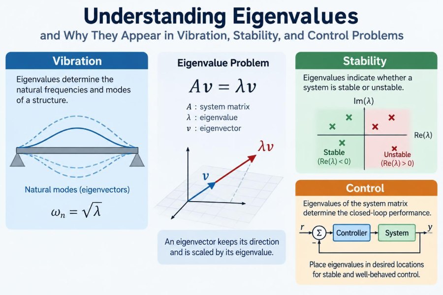
For a matrix A, an eigenvector v and eigenvalue λ satisfy:
Av = λv
This says that applying the matrix to v produces the same direction again, multiplied by a number λ. The vector may stretch, shrink, reverse, or—when complex numbers are involved—participate in a rotating oscillation pattern.
That special preservation of pattern is why eigenvalues appear so often in engineering. Physical systems are rarely affected in just one coordinate at a time; matrices describe coupled effects, while eigenvectors reveal the system’s independent modes.
🧭 Matrices as transformations, not just arrays
Students often first meet a matrix as a rectangular arrangement of numbers used in simultaneous equations. In engineering, it is more useful to see a matrix as an operation that maps one state into another.
A two-dimensional matrix can rotate, shear, stretch, or reflect a vector. Most input directions change direction after the transformation. An eigenvector is exceptional: it lies along a direction that the transformation leaves aligned with itself.
For a mechanical model, the “vector” may represent displacements. In an electrical circuit it may contain voltages and currents. In a control model it may collect positions, speeds, temperatures, or other state variables.
➡️ Why eigenvectors matter alongside eigenvalues
An eigenvalue alone tells part of the story: a scale factor, growth rate, or modal parameter. The associated eigenvector tells which coordinated pattern of motion or state change has that behavior.
Consider two masses connected by springs. One mode may have both masses moving in the same direction together. Another may have them moving in opposite directions. These shapes are eigenvectors; their corresponding natural frequencies are obtained from eigenvalues.
In large systems, the eigenvector is often called a mode shape. It shows where movement is strongest, where a node occurs, and which components participate substantially in a particular mode.
🧮 A small numerical example
Take the matrix:
A = [ 3  1 ]
    [ 0  2 ]
Because this matrix is triangular, its eigenvalues are visible on the diagonal: λ = 3 and λ = 2. For λ = 3, the vector [1, 0]ᵀ is an eigenvector because multiplying by A gives [3, 0]ᵀ.
For λ = 2, an eigenvector is [−1, 1]ᵀ. The matrix changes its magnitude but does not alter its line of action. This small example contains the entire definition, though real engineering matrices are usually larger and physically structured.
🧾 The characteristic equation
To find eigenvalues, rearrange the defining equation:
Av = λv
(A − λI)v = 0
Here, I is the identity matrix. A nonzero vector v can solve this equation only when the matrix A − λI is singular, meaning it has no inverse.
The determinant condition is therefore:
det(A − λI) = 0
This is the characteristic equation. Its roots are the eigenvalues. For an n × n matrix, it is generally a polynomial of degree n.
📐 Finding eigenvectors after the roots
Once an eigenvalue is known, substitute it into (A − λI)v = 0 and solve the resulting homogeneous linear equations. The nonzero solutions form the eigenspace for that eigenvalue.
Eigenvectors can be multiplied by any nonzero constant without changing their physical pattern. A vibration mode shape, for example, can be scaled so that its largest component is one, or normalized to satisfy a mass-related convention.
This freedom means that absolute numbers in a plotted mode shape are not necessarily physical amplitudes. The meaningful information is the relative motion between components.
🎵 Natural frequencies in vibration systems
A structure has preferred ways of vibrating after it is disturbed. These are its natural modes. A tuning fork, a machine shaft, a building floor, and a spacecraft panel all have them.
For an undamped linear system with mass matrix M and stiffness matrix K, free vibration is commonly written as:
Mẍ + Kx = 0
Assuming a harmonic motion pattern leads to the generalized eigenvalue problem:
Kφ = ω²Mφ
The values ω² are eigenvalues, ω are natural circular frequencies, and φ are mode shapes.
🪕 The mass–spring intuition
A single mass on a spring has one natural frequency, determined by its stiffness and mass. A two-mass system has more possibilities because the masses can move in coordinated but different patterns.
In a simple hypothetical pair of equal masses and springs, one mode may move both masses together. Another may move them against each other, stretching a connecting spring more strongly. The latter is usually associated with greater restoring force and hence a higher natural frequency.
Eigenvalue analysis turns this intuition into a scalable method. Instead of trying to guess motion patterns for a model with hundreds of degrees of freedom, software calculates its modes systematically.
🏗️ Why resonance is an eigenvalue problem
Resonance occurs when external excitation is near a natural frequency and the system can absorb energy efficiently. The amplitude then depends not only on frequency, but also on damping, forcing location, duration, and the match between the applied force and a mode shape.
Eigenvalues identify frequencies worth examining before a machine or structure is built. They do not, by themselves, predict the final response amplitude under every operating condition.
A rotating machine may have a forcing frequency linked to its rotational speed. Designers compare that excitation range with calculated natural frequencies and seek adequate separation, damping, or changes in stiffness and mass.
🛑 Damping changes the picture
Real structures lose energy through material effects, joints, fluids, friction, and dedicated dampers. Damping makes vibration problems more realistic, but it also moves the mathematics from simple frequency values to complex eigenvalues.
A typical dynamic model is:
Mẍ + Cẋ + Kx = 0
where C is the damping matrix. The real part of a complex eigenvalue is associated with decay or growth, while the imaginary part is associated with oscillation. Interpreting these values carefully is central to stability analysis.
🌊 Complex eigenvalues are not a complication to avoid
Complex eigenvalues often alarm learners because physical displacement and voltage are real quantities. The complex notation is a compact way to represent oscillation and phase relationships.
For a continuous-time state model, an eigenvalue of the form σ ± jω corresponds to behavior resembling an oscillation at angular frequency ω, with an envelope governed by σ. If σ is negative, the envelope decays; if positive, it grows.
Complex conjugate pairs arise for real-valued system matrices. Their combined contribution produces a real physical response.
📉 Stability in continuous-time systems
A linear time-invariant state-space model is often written as:
ẋ = Ax
Its eigenvalues are commonly called poles of the state matrix. For an unforced continuous-time system, asymptotic stability requires every eigenvalue of A to have a strictly negative real part.
The reason is physical as well as mathematical. Each modal contribution includes a factor related to e^(λt). A negative real part decays with time, a positive real part grows, and a zero real part requires closer examination.
⚖️ Stable, marginal, and unstable behavior
| Eigenvalue location | Typical free response | Engineering interpretation |
|---|---|---|
| Negative real part | Decays | Disturbance tends to die away |
| Negative real part with nonzero imaginary part | Decaying oscillation | Stable but potentially underdamped |
| Zero real part | Persistent or delicate behavior | Marginal case; model details matter |
| Positive real part | Grows | Unstable linearized behavior |
For nonlinear systems, eigenvalues of a linearization describe behavior near an operating point, not necessarily far from it. That limitation is crucial: a locally stable model does not guarantee acceptable behavior across every possible condition.
🕒 Discrete-time stability uses a different boundary
Digital controllers, sampled data systems, and iterative numerical models are often written as:
x[k+1] = Ax[k]
For these systems, stability depends on whether every eigenvalue lies inside the unit circle in the complex plane: |λ| < 1. Repeated multiplication by such a factor causes the mode to shrink from sample to sample.
This differs from continuous time, where the relevant boundary is the imaginary axis. Mixing up these two tests is a common and consequential error.
🗺️ The complex plane gives a fast diagnostic
Plotting eigenvalues can immediately reveal the dominant dynamic tendencies of a system. In continuous time, the vertical axis indicates oscillatory content and the horizontal axis indicates growth or decay.
Modes close to the imaginary axis decay slowly. Even if technically stable, they can produce long settling times, noticeable ringing, or poor disturbance rejection. Modes far to the left tend to decay more quickly, though forcing them there through control can create other costs.
In discrete time, the equivalent visual test is distance from the origin. Points close to the unit circle often indicate slowly decaying sampled behavior.
🎛️ State-space models connect mathematics to control
A common control model is:
ẋ = Ax + Bu
y = Cx + Du
The state vector x holds internal variables, u is the input, and y is the measured output. The matrix A describes the system’s natural internal evolution when inputs are absent.
Therefore, eigenvalues of A reveal the open-loop dynamics. They answer questions such as: Will a disturbance fade? Is there an oscillatory mode? Which response is slow enough to matter during operation?
🧲 Feedback changes closed-loop eigenvalues
With state feedback u = −Kx, the closed-loop model becomes:
ẋ = (A − BK)x
The eigenvalues of A − BK determine the closed-loop modal behavior. In suitable systems, selecting the gain matrix K can place eigenvalues in locations that provide desired response speed and damping.
This is the basis of pole placement. It is powerful, but not a license to choose arbitrarily fast poles: actuator limits, sensor noise, unmodeled dynamics, and robustness constrain practical designs.
🚁 A control example: correcting a tilt disturbance
Imagine a simplified drone attitude model. A small tilt produces angular motion; motors generate torques intended to correct it. Without adequate feedback, the tilt may persist, oscillate, or increase.
The open-loop eigenvalues describe those natural tendencies near the hover condition. A feedback controller shifts the closed-loop eigenvalues so that a small tilt returns toward zero with an acceptable compromise between speed and overshoot.
The analysis does not replace flight testing. It provides a disciplined starting point and highlights modes that may be difficult to control before full hardware trials.
🧩 Coupling is why component-by-component reasoning fails
Engineering systems are often coupled. Moving one coordinate can affect several others: a vehicle’s lateral motion couples with yaw, an aircraft’s pitch couples with speed, and a flexible beam’s modes involve many points moving together.
Looking only at diagonal entries of a model can miss the behaviors created by those interactions. Eigenvalue analysis incorporates the whole matrix and exposes coordinated patterns that no individual equation fully describes.
This is especially valuable when a small coupling term shifts a lightly damped mode toward instability.
🏭 Modal analysis in real design workflows
Finite element models convert a complex structure into many connected elements and degrees of freedom. The resulting mass and stiffness matrices can be very large, yet the lowest modes are often most relevant to operating loads and human perception.
A typical workflow includes:
- Define geometry, materials, supports, and connections.
- Assemble mass and stiffness representations.
- Compute selected natural frequencies and mode shapes.
- Inspect whether the shapes and frequencies are physically plausible.
- Compare critical modes with forcing sources and design requirements.
- Refine the model or alter the design where necessary.
The calculation is not the endpoint. Boundary conditions, joint stiffness, added equipment, and uncertain material properties can strongly influence useful results.
🔧 Boundary conditions can dominate the answer
A beam fixed at one end behaves very differently from the same beam simply supported or free at both ends. These constraints change the admissible mode shapes and therefore the eigenvalues.
In practice, “fixed” supports may have flexibility, bolted joints may slip slightly, and attached cables or piping may add mass and restraint. A mathematically precise eigenvalue from an unrealistic boundary assumption is still a poor design guide.
When test data are available, engineers often use them to update uncertain model parameters rather than assuming the first idealized model is final.
🧱 Repeated eigenvalues and special cases
An eigenvalue may occur more than once. This is called an algebraic multiplicity greater than one. Symmetric structures can produce repeated or closely spaced modes, sometimes with different independent mode shapes at the same frequency.
Not every matrix has enough independent eigenvectors to form a complete eigenvector basis. Such a matrix is called defective. The usual diagonalization shortcut then fails, and a more careful treatment is needed.
These cases are not merely algebraic curiosities. Nearly repeated modes can mix under small physical changes, making mode identification and model correlation more sensitive.
🪞 Symmetric matrices provide a valuable simplification
Many undamped structural models lead to symmetric mass and stiffness matrices. Under appropriate conditions, this gives real natural frequencies and mode shapes with useful orthogonality properties.
Mass orthogonality allows modal coordinates to separate a coupled physical model into simpler modal equations. Each retained mode can then be analyzed much like a single oscillator, while the full response is reconstructed from their combination.
Non-symmetric systems also occur frequently, particularly with aerodynamic effects, gyroscopic terms, nonconservative forces, and general control models. Their modes need more care and may not have the same convenient properties.
🧠 Modal coordinates simplify coupled motion
Suppose physical displacement is represented approximately by x = Φq, where the columns of Φ are selected mode shapes and q contains modal coordinates. The transformation replaces many physical coordinates with amplitudes of meaningful vibration patterns.
For well-behaved structural systems, this can reduce a complicated model to several nearly independent modal equations. Engineers can focus on the few modes within the frequency range of interest.
Truncating higher modes is efficient, but it must be justified. High-frequency modes may still matter near local loads, sharp transients, sensors, actuators, or control bandwidth.
📏 Units and scaling deserve attention
Eigenvalues do not always share the same units. In the vibration relation Kφ = ω²Mφ, the eigenvalue has units of inverse time squared, so taking its square root produces angular frequency.
For ẋ = Ax, eigenvalues have units of inverse time when state variables are consistently defined. In a discrete-time model, eigenvalues are dimensionless multipliers per sample.
Numerical scaling matters too. If one state is measured in micrometres and another in kilometres, poorly scaled matrices can make computations and interpretation less reliable. Nondimensionalization or thoughtful variable scaling can help.
💻 What numerical software actually computes
For small matrices, hand calculations teach the mechanism. For realistic models, engineers use numerical algorithms rather than expanding large determinants, which is inefficient and numerically fragile.
Software may return complex eigenvalues, normalized eigenvectors, and an ordering chosen by magnitude or real part. Always inspect documentation: normalization, ordering, and treatment of generalized problems vary by tool.
A result should be checked against physics. Rigid-body modes near zero frequency, expected symmetry, plausible mode shapes, and convergence under mesh refinement are often more revealing than a solver’s successful completion message.
⚠️ Common mistakes in eigenvalue interpretation
- Confusing a mode shape with a forced-response shape: operating motion depends on excitation and damping as well as natural modes.
- Using frequency alone: a natural frequency near an excitation is a warning, not a complete resonance prediction.
- Ignoring units: angular frequency in radians per second is not the same number as frequency in hertz.
- Applying the wrong stability rule: continuous-time and discrete-time models use different stability regions.
- Trusting unstable-looking numerical noise: very small positive real parts can arise from modeling or numerical tolerances and require investigation.
- Assuming linear results cover every amplitude: nonlinearities can change frequencies, damping, and stability away from the operating point.
🧪 Validation turns a calculation into engineering evidence
Eigenvalue results are predictions from a model. Validation asks whether the model represents the physical system well enough for the intended decision.
Experimental modal analysis can estimate frequencies, damping, and mode shapes from measured responses. Control engineers may compare predicted poles and time responses with data from carefully designed tests.
Agreement is rarely perfect. The useful question is whether discrepancies affect the modes, operating ranges, and safety margins that matter for the design.
🔄 Sensitivity explains why small changes can matter
Changing mass, stiffness, damping, feedback gain, or operating condition can move eigenvalues. Tracking those movements helps identify which parameter has the strongest influence on a troublesome mode.
Adding stiffness often raises a structural natural frequency, but the effect depends on where the stiffness is added and which mode is considered. Adding mass can lower some frequencies, yet it can also alter mode shapes and coupling.
In control design, a gain increase may move a pole toward faster response while reducing damping or increasing sensitivity to measurement noise. Eigenvalue movement should therefore be interpreted with other performance measures, not in isolation.
🧭 A practical checklist for new problems
When eigenvalues appear in a new engineering model, start by identifying what the matrix represents. Then connect the mathematical result to the physical system rather than treating roots as detached numbers.
- Is the model continuous-time, discrete-time, static, or a vibration eigenproblem?
- What are the state variables or degrees of freedom?
- What do the eigenvalue units mean in this formulation?
- Which eigenvalues are closest to a stability boundary or operating excitation?
- Do the eigenvectors resemble physically credible patterns?
- Which assumptions about damping, supports, sensors, loads, or linearization limit the conclusion?
These questions prevent many errors before any design decision is made.
🎯 The unifying principle
Vibration, stability, and control problems all involve a system evolving under coupled rules. Eigenvalues identify the system’s characteristic rates and frequencies; eigenvectors identify the patterns in which those characteristics occur.
In vibration, they reveal natural frequencies and mode shapes. In stability, they show whether small disturbances decay, persist, or grow. In control, they provide a language for shaping closed-loop dynamics through feedback.
The mathematics is the same because the underlying question is the same: what behaviors are built into this coupled system, and what happens to each behavior over time?
Eigenvalues turn a complicated coupled model into identifiable dynamic modes, giving engineers a practical bridge from equations to physical behavior. Learn to read both the values and their vectors, and vibration, stability, and control problems become far less mysterious. 📐⚙️📈