
A simulation can run without errors, return a neat column of numbers, and still point an engineer in the wrong direction. A structural model may predict an implausibly large displacement; a control algorithm may react wildly to a tiny sensor fluctuation; a curve-fitting routine may produce coefficients that change every time the data are updated.
These failures are often not programming mistakes. They can arise because the mathematical problem itself is unusually sensitive: a small uncertainty in the input creates a much larger uncertainty in the output.
This matters wherever measured data, finite-precision arithmetic, and computational models meet—which is to say, in much of engineering. Numerical stability is the discipline of recognizing that sensitivity and choosing formulations and algorithms that do not amplify it unnecessarily.
The goal is not to make every answer exact. Real measurements are never exact. The goal is to produce answers whose uncertainty is understood, proportionate, and fit for the decision being made.
🧭 What “ill-conditioned” actually means
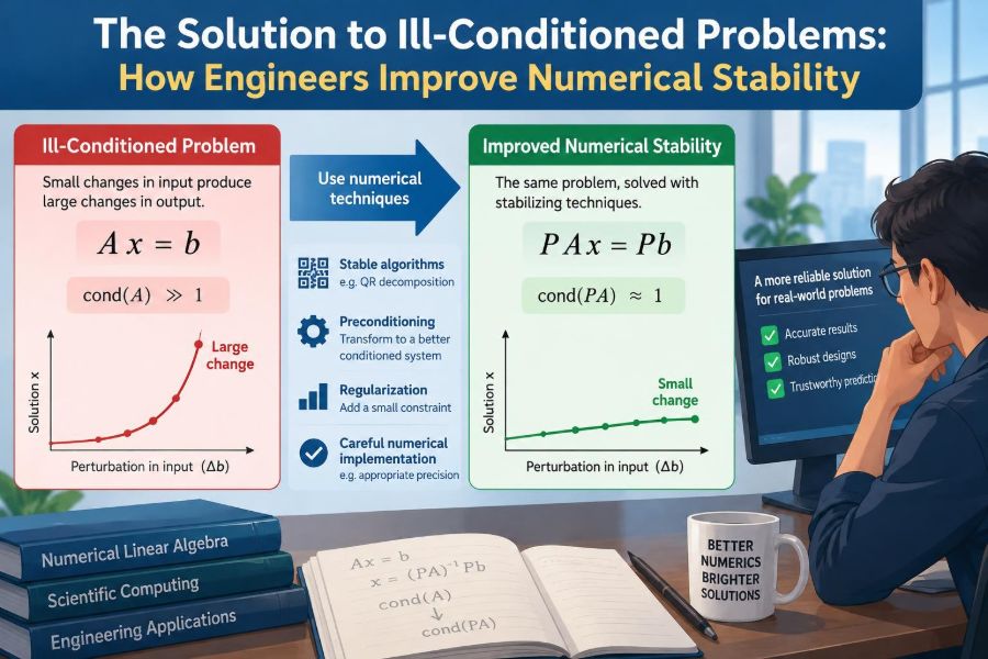
A problem is well-conditioned when small relative changes in its inputs cause comparably small relative changes in its output. It is ill-conditioned when a small input change can cause a disproportionately large output change.
Conditioning is a property of the underlying mathematical problem, not of one particular program. If two nearly identical sets of experimental measurements imply dramatically different parameter estimates, the estimation problem may be ill-conditioned even if the code is flawless.
🔍 A simple sensitivity example
Consider calculating the difference between two lengths, 10.000 m and 9.999 m. The result is 0.001 m. If each original measurement has a small uncertainty, say in its last few digits, that uncertainty may be large compared with the tiny difference.
The subtraction is mathematically valid, but the result is sensitive because it depends on separating two almost equal quantities. This familiar situation previews a major numerical hazard: loss of significant information through cancellation.
📏 Condition numbers quantify the risk
A condition number measures how strongly relative input errors may be amplified into relative output errors. A condition number near one generally indicates modest sensitivity. A very large condition number warns that even good input data may not support many trustworthy output digits.
For a square matrix A, a common matrix condition number is written as κ(A) = ‖A‖‖A⁻¹‖, using a chosen compatible norm. In practice, software often estimates this value rather than explicitly computing the inverse.
🧮 Conditioning is not algorithmic stability
Two ideas must be kept separate. Conditioning asks whether the problem is sensitive. Numerical stability asks whether an algorithm introduces or magnifies avoidable numerical error while solving it.
A stable algorithm can give the best realistically attainable answer to an ill-conditioned problem, but it cannot create information absent from the data. Conversely, an unstable method can damage an otherwise well-conditioned problem. Good engineering requires attention to both.
| Question | Conditioning | Stability |
|---|---|---|
| What is being assessed? | The mathematical problem | The computational method |
| Main source of difficulty | Input sensitivity | Roundoff and algorithmic error |
| Typical response | Improve data or reformulate the model | Choose a better algorithm or implementation |
💻 Why floating-point arithmetic matters
Computers represent most real numbers with a finite number of binary digits. Many familiar decimal values cannot be represented exactly, and arithmetic results must be rounded to the nearest representable number.
These tiny roundoff errors are usually harmless. They become consequential when an algorithm repeatedly magnifies them, when values have vastly different scales, or when the original problem is already ill-conditioned. More digits help only up to the limit imposed by the data and formulation.
➖ Catastrophic cancellation in subtraction
When nearly equal floating-point values are subtracted, their leading matching digits disappear. The remaining digits may contain little reliable information. This is called catastrophic cancellation, although the operation itself is not always avoidable or wrong.
For example, the expression √(x² + 1) − x is problematic for very large positive x. A numerically preferable equivalent form is 1/(√(x² + 1) + x). Rationalizing the expression avoids subtracting nearly equal terms.
🧱 Linear systems are a central engineering case
Many models lead to Ax = b: circuit equations, finite-element equilibrium, heat-flow networks, and regression problems all fit this form. If the columns of A are nearly linearly dependent, then different combinations of unknowns can explain the equations almost equally well.
The resulting solution x can then be highly sensitive to small changes in b or A. A solver returning a vector is not evidence that the vector is physically meaningful; residuals and conditioning must also be examined.
📐 Near-dependent columns reveal weak information
Imagine estimating two material effects from tests where both effects change the measured response in almost the same pattern. The model may struggle to determine which effect caused what portion of the response.
Mathematically, the corresponding matrix columns are nearly parallel. Experimentally, the tests do not provide enough independent information. This is often an identifiability issue, not a computational defect.
🔺 Why directly inverting a matrix is usually a poor plan
It is tempting to rewrite Ax = b as x = A⁻¹b and calculate the inverse. For solving one system, this usually does extra work and may introduce unnecessary numerical error. Forming an inverse can also obscure better diagnostics and structure.
Prefer a factorization or a dedicated linear-system solver. Use an inverse when the inverse itself is genuinely required, and even then consider whether a factorization can serve the intended calculation more reliably.
🧩 LU factorization and pivoting
For many square systems, LU factorization expresses a matrix as lower- and upper-triangular factors. Solving triangular systems is efficient, so this is a practical foundation for repeated solves.
Pivoting rearranges rows, and sometimes columns, to avoid dividing by a tiny intermediate value. Partial pivoting is a standard safeguard in general dense problems. It does not cure ill-conditioning, but it often prevents the algorithm from making an avoidable instability worse.
📉 QR factorization for least squares
When there are more observations than unknowns, engineers commonly solve a least-squares problem: find x that makes ‖Ax − b‖ small. A fragile route forms the normal equations AᵀAx = Aᵀb.
That route squares the condition number in a common norm, potentially making sensitivity much worse. QR factorization works more directly with A and is usually the safer standard choice for ordinary least-squares computation.
🪜 Singular value decomposition exposes the geometry
The singular value decomposition, or SVD, writes a matrix in directions that are independently stretched or compressed. Very small singular values identify directions in parameter space that the data barely constrain.
This makes SVD especially valuable for diagnosing rank deficiency, solving difficult least-squares problems, and understanding why fitted parameters are unstable. It can cost more than simpler factorizations, so it is often used selectively where reliability and diagnosis justify that cost.
🧪 Residuals alone do not validate a solution
A residual measures how well a computed solution satisfies the supplied equations: r = b − Ax. A small residual is useful, but it does not guarantee that x is close to the true solution.
In an ill-conditioned system, many substantially different solutions may produce small residuals. Check the residual, estimated conditioning, scale of variables, and whether the resulting values make physical sense. Each answers a different question.
🔄 Backward error offers a practical perspective
A method is often called backward stable when its computed answer is the exact solution to a nearby problem, with perturbations comparable to unavoidable roundoff. This is a powerful standard because real inputs already contain uncertainty.
Backward stability does not promise a small forward error—the difference between computed and exact solutions—when the problem is ill-conditioned. It does mean the algorithm has not demanded unrealistically precise input information.
⚖️ Scaling changes the numerical landscape
Variables in engineering models can differ by many orders of magnitude: pressure in pascals, a geometric tolerance in micrometres, and an elastic modulus in gigapascals. Such mismatches can make intermediate computations poorly behaved.
Scale variables and equations so typical quantities are near comparable magnitudes where practical. Nondimensionalization, unit-aware transformations, and row or column scaling can improve numerical behavior and make solver tolerances meaningful. Scaling does not alter the physical solution when applied consistently.
🌡️ Nondimensionalization adds physical clarity
Nondimensionalization replaces dimensional variables with ratios to characteristic scales, such as temperature relative to a reference difference or distance relative to a device length. It often reveals which physical effects actually govern a system.
Numerically, it reduces extreme magnitudes and makes coefficients easier to compare. It also prevents a solver tolerance from being accidentally interpreted across incompatible units. The chosen scales should be physically justified, not selected merely to make numbers look tidy.
🧰 Preconditioning helps iterative solvers
Large sparse systems are frequently solved iteratively rather than by dense factorizations. A preconditioner transforms the system into one that has the same solution but is easier for the iterative method to solve.
An effective preconditioner clusters relevant eigenvalues or reduces troublesome scaling, so convergence takes fewer iterations. Designing one depends on the physics and matrix structure; a preconditioner that is cheap but weak may save little, while a very elaborate one may cost more than it returns.
🕸️ Preserve sparsity in large models
Finite-element and network models often create sparse matrices: most entries are zero because each component interacts only with nearby components. Treating these matrices as dense wastes memory and computation.
Sparse orderings, factorization methods, and iterative solvers preserve this structure. They also affect stability indirectly, because excessive fill-in can make a theoretically suitable method impractical at the scale where careful numerical treatment is most needed.
🧷 Regularization trades variance for bias
When data cannot distinguish among many plausible parameter vectors, regularization deliberately adds a preference for solutions with a useful property, such as small magnitude or smooth variation. Ridge regression is a familiar example.
This stabilizes estimates by reducing sensitivity to noise, but it introduces bias: the result is no longer simply the unconstrained best fit. The regularization strength should reflect domain knowledge, validation procedures, or decision consequences—not an arbitrary default.
🧯 Truncated SVD discards unreliable directions
In an SVD-based solution, dividing by a tiny singular value strongly amplifies noise. Truncated SVD avoids this by omitting directions associated with sufficiently small singular values.
The trade-off is explicit. Fine detail in poorly observed directions is lost, but the result becomes less dominated by measurement noise. This is appropriate only when those discarded directions are genuinely unsupported by the data, rather than merely inconvenient.
📈 Polynomial fitting can become unexpectedly fragile
High-degree polynomial interpolation at evenly spaced points may oscillate severely, especially near the ends of an interval. This is a classic example where a mathematically valid approximation can be a poor numerical or modeling choice.
Rescaling the input range, using orthogonal polynomial bases, choosing carefully placed nodes, or fitting splines can produce more dependable behavior. A higher-degree curve is not automatically a more informative model of measured engineering data.
🧭 Choose a model no more flexible than the evidence
Ill-conditioning often appears because a model has more adjustable freedom than the experiment can support. Fitting many correlated parameters to limited, noisy observations can produce excellent apparent fit and unstable interpretation.
Before changing solvers, ask whether each parameter has a distinct observable effect. Simplifying the model, collecting measurements under more varied operating conditions, or fixing a known parameter may improve the problem more than any numerical trick.
📡 Improve the experiment, not only the computation
Numerical methods cannot recover distinctions that an experiment never measured. If two parameters are confounded, change test conditions so their predicted effects separate: vary loads, frequencies, geometries, or operating regimes where physically appropriate.
Repeated measurements reduce random variation in some contexts, but repetition alone does not create independent information. Experimental design should seek informative variation, reliable calibration, and measurements at scales that can meaningfully resolve the quantities of interest.
🧭 Sensitivity analysis identifies the leverage points
Sensitivity analysis asks how outputs respond when inputs or parameters are perturbed. Local sensitivities use derivatives near a nominal point; broader methods explore changes over a stated range of assumptions.
Use it to find which dimensions, material properties, boundary conditions, or sensor readings dominate uncertainty. This guides effort toward the measurements worth improving and away from inputs whose precision has little effect on the engineering decision.
✅ Validate with perturbation tests
A useful practical check is to perturb credible inputs by their expected uncertainty and observe how much the outputs move. Repeat calculations with alternative reasonable scalings, solver tolerances, or formulations when possible.
If conclusions change substantially under tiny credible perturbations, report that sensitivity rather than presenting a single number with false confidence. For safety-critical or high-cost decisions, independent model checks and domain review are especially valuable.
🔢 Precision is a tool, not a cure
Using higher-precision arithmetic can reduce roundoff error and may be justified in sensitive calculations, verification work, or specialized scientific software. It cannot repair noisy measurements, a structurally unidentifiable model, or a fundamentally ill-conditioned inverse problem.
Higher precision also costs time and memory. First improve the formulation, scaling, algorithm, and data design. Then use additional precision when analysis shows that arithmetic roundoff, rather than input uncertainty, limits the result.
🚫 Common numerical habits that create trouble
- Solving by explicitly computing a matrix inverse when a factorization is available.
- Using normal equations by default for a poorly conditioned least-squares problem.
- Comparing results only through residuals and ignoring parameter uncertainty.
- Mixing units or leaving variables at wildly different scales.
- Reporting many digits because software printed them.
- Adding regularization without explaining the assumption it imposes.
These habits are tempting because they can produce an answer quickly. Reliable numerical work asks what that answer can legitimately support.
🧾 Report uncertainty and numerical choices clearly
A technical result is more useful when readers know the assumptions behind it. Record data sources and units, scaling choices, solver and factorization, stopping criteria, estimated conditioning where available, and the treatment of constraints or regularization.
Round reported values to a precision consistent with uncertainty. A concise uncertainty range, sensitivity statement, or warning about weakly identified parameters is often more honest and more actionable than a long decimal expansion.
🛠️ A practical workflow for difficult calculations
- Define the physical question and the accuracy needed for the decision.
- Check units, magnitudes, data quality, and model assumptions.
- Scale or nondimensionalize variables where appropriate.
- Estimate conditioning and inspect rank or singular values for sensitive systems.
- Select a stable method suited to the matrix structure and task.
- Validate with residuals, perturbations, physical checks, and independent comparisons where possible.
- Communicate uncertainty, limitations, and any regularizing assumptions.
This workflow prevents a common failure mode: spending effort tuning a solver before understanding whether the model and measurements can answer the question.
🏁 The core principle: manage sensitivity, not just error
Ill-conditioned problems are not always mistakes. They often reveal something real: measurements lack independent information, a chosen representation is fragile, or a desired level of detail exceeds what the system can resolve.
Engineers improve numerical stability by combining sound mathematics with physical judgment: reformulate cancellation-prone expressions, choose stable factorizations, scale models, preserve structure, regularize transparently, and design measurements that distinguish the effects they seek to estimate.
The most reliable numerical answer is not the one with the most digits; it is the one whose sensitivity, assumptions, and uncertainty are understood well enough to support the engineering decision.