📡 How the Fast Fourier Transform Analyzes Complex Signals Efficiently

Many signals in the real world look complicated when viewed over time. A piece of music contains many notes at once, a vibration sensor records multiple mechanical frequencies, an ECG captures changing electrical activity from the heart, and a wireless receiver may detect several overlapping radio signals. 📈🎵

At first glance, these signals can appear chaotic. However, many complex signals are really combinations of simpler oscillations occurring at different frequencies.

The mathematical tool used to separate a signal into these frequency components is the Fourier transform.

The problem is that directly computing a Fourier transform for a large digital signal can require enormous amounts of calculation. This is where the Fast Fourier Transform, or FFT, becomes extremely important.

The FFT is not a different transform. Instead, it is a highly efficient family of algorithms for computing the Discrete Fourier Transform (DFT).

By reorganizing the calculations and eliminating repeated work, the FFT can reduce a computation that might otherwise require millions or billions of operations into something dramatically more manageable. ⚡🧠

That efficiency is why the FFT has become one of the most important algorithms in digital signal processing.

🌊 What Is a Signal?

A signal is any quantity that varies and carries information.

Examples include:

🎤 Sound pressure measured by a microphone
📡 Radio waves received by an antenna
🌡️ Temperature changing over time
❤️ Electrical activity measured by an ECG
⚙️ Vibrations measured on industrial machinery
💡 Light intensity detected by an optical sensor

A digital system normally represents a signal as a sequence of numerical samples.

For example, an audio recording might contain:

0.15, 0.22, 0.18, -0.04, -0.31, -0.48...

Each number represents the signal’s amplitude at a particular moment.

Looking at those numbers tells us how the signal changes over time.

This is known as the time domain.

⏱️ Time Domain vs. Frequency Domain

The same signal can also be described according to which frequencies it contains.

This alternative representation is called the frequency domain.

Imagine hearing a piano chord consisting of three notes.

In the time domain, the sound waveform may look complicated because all three notes are mixed together.

In the frequency domain, however, you might see three strong peaks corresponding to the frequencies of the individual notes. 🎹

Conceptually:

Time-domain waveform ➡️ Fourier transform ➡️ Frequency spectrum

Instead of asking:

“How does the signal change over time?”

the frequency-domain representation asks:

“How much of each frequency is present in the signal?”

Both descriptions contain information about the same underlying signal, but they make different properties easier to see.

🎵 Complex Signals as Combinations of Sinusoids

Fourier analysis is based on a remarkable idea: many signals can be represented as combinations of sinusoidal waves.

A sinusoidal wave may be written conceptually as:

Amplitude × sin(frequency × time + phase)

Each sinusoid has important properties:

Frequency – how quickly it oscillates
Amplitude – how strong it is
Phase – where it is within its cycle

Imagine a signal containing three sine waves:

100 Hz
300 Hz
800 Hz

When combined in the time domain, the result may look irregular.

Fourier analysis separates the mixture and reveals those individual components.

Instead of one confusing waveform, the frequency spectrum might show:

100 Hz → strong
300 Hz → medium
800 Hz → weak

This makes signal analysis much easier.

🧮 What Is the Discrete Fourier Transform?

For digital signals, the relevant operation is usually the Discrete Fourier Transform, or DFT.

Suppose a digital signal contains N samples.

The DFT examines those samples and calculates how strongly different frequencies contribute to the signal.

The result is a sequence of frequency-domain values.

Each output value is generally a complex number, containing information about both amplitude and phase.

A simplified DFT formula is:

X[k] = Σ x[n] e^(-j2πkn/N)

where:

x[n] represents the input samples
X[k] represents the frequency-domain outputs
N is the number of samples
j represents the imaginary unit
k identifies a frequency bin

The equation may look intimidating, but conceptually the DFT compares the input signal with many possible sinusoidal patterns.

It asks:

“How much does this frequency appear in the signal?”

📦 What Is a Frequency Bin?

A DFT does not normally report every possible frequency.

Instead, it divides the analyzed frequency range into discrete positions known as frequency bins.

If the sampling rate is Fs and the transform contains N samples, the spacing between frequency bins is:

Frequency resolution = Fs / N

Suppose:

Sampling rate = 48,000 samples per second

and:

N = 48,000 samples

Then the spacing is:

48,000 / 48,000 = 1 Hz

The resulting frequency spectrum has bins separated by approximately 1 Hz.

Larger sample windows can therefore provide finer frequency resolution.

🐢 Why a Direct DFT Can Be Slow

Computing the DFT directly requires evaluating many combinations of input samples and output frequencies.

For N input samples, there are approximately N output frequency bins.

Each output may require calculations involving all N samples.

This means a straightforward DFT requires roughly:

N × N = N²

operations.

Computer scientists describe this complexity as:

O(N²)

For small inputs, this may not be a serious problem.

For large inputs, however, the amount of computation becomes enormous.

Suppose:

N = 1,000,000 samples

A direct DFT could require on the order of:

1,000,000² = 1 trillion

basic computational steps.

That is far too expensive for many real-time applications.

⚡ Enter the Fast Fourier Transform

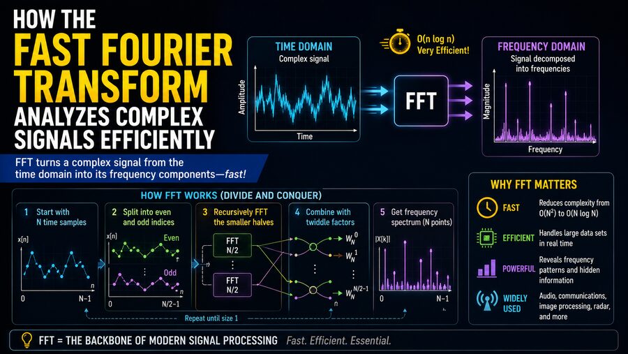
The Fast Fourier Transform dramatically reduces the amount of work required.

A typical FFT requires roughly:

O(N log N)

operations instead of:

O(N²)

This difference becomes enormous as N grows.

For about one million samples:

A direct DFT might require roughly:

10¹²-scale operations

while an FFT may require only on the order of:

20 million computational stages or combinations, depending on how operations are counted.

The exact numbers vary, but the improvement is dramatic.

This efficiency transformed Fourier analysis from a mathematically powerful but computationally expensive operation into something that can be performed routinely on phones, computers, embedded processors, and scientific instruments. 📱💻

🧩 How Does the FFT Become Faster?

The key idea is divide and conquer.

Instead of calculating the entire DFT directly, the FFT breaks the problem into smaller DFTs.

These smaller transforms can then be combined efficiently.

A famous FFT method is the Cooley-Tukey algorithm.

One common version splits the original signal into:

Samples at even-numbered positions
Samples at odd-numbered positions

Suppose we have eight samples:

x0, x1, x2, x3, x4, x5, x6, x7

The algorithm separates them into:

Even: x0, x2, x4, x6
Odd:  x1, x3, x5, x7

Instead of computing one eight-point DFT directly, it computes two four-point DFTs.

Those four-point transforms can then be broken into two-point transforms.

The process continues recursively.

Conceptually:

8-point DFT

⬇️

Two 4-point DFTs

⬇️

Four 2-point DFTs

⬇️

Combine results efficiently

This decomposition eliminates a great deal of repeated calculation.

🦋 What Is the FFT Butterfly?

Many FFT diagrams contain a distinctive crossing pattern called a butterfly. 🦋

A butterfly is a small computational structure that combines intermediate values.

A simplified butterfly takes two values and calculates combinations such as:

A + WB

and:

A − WB

where W is a complex coefficient known as a twiddle factor.

By repeatedly applying butterfly operations, the FFT combines the results of smaller transforms into the complete frequency spectrum.

Large FFTs contain many butterfly stages arranged systematically.

🔄 What Are Twiddle Factors?

Twiddle factors are complex-number coefficients representing rotations in the complex plane.

They are based on expressions such as:

e^(-j2πk/N)

These factors encode the phase relationships needed when combining smaller Fourier transforms.

A major source of FFT efficiency comes from recognizing that many of these values repeat or are mathematically related.

Instead of recomputing every quantity independently, the algorithm reuses structure.

This is one of the central reasons FFT algorithms are so much faster than the straightforward DFT.

📈 What Does the FFT Output Look Like?

The FFT produces complex values.

Each complex result contains information about both the strength and phase of a frequency component.

From each result, we can calculate:

📊 Magnitude

The magnitude indicates how strongly that frequency is present.

A magnitude spectrum may show peaks like:

100 Hz  █████████
300 Hz  █████
800 Hz  ██

🔄 Phase

The phase tells us where the corresponding sinusoidal component is positioned within its cycle.

Both magnitude and phase are important if we want to reconstruct the original signal accurately.

🎤 Example: Analyzing an Audio Recording

Imagine recording a singer holding a musical note.

The microphone captures a complicated waveform.

The signal may contain:

The fundamental note
Harmonics
Room reflections
Background noise

Running an FFT on a short segment might reveal:

220 Hz – fundamental frequency

440 Hz – second harmonic

660 Hz – third harmonic

Additional smaller peaks might correspond to other harmonics or noise.

This is far more informative than simply looking at the raw waveform.

Audio software can use this information for:

Pitch detection
Equalization
Noise reduction
Music visualization
Speech analysis
Instrument identification

🎧 FFTs are therefore fundamental to modern digital audio.

🪟 Why Signals Are Often Windowed Before an FFT

An FFT normally analyzes a finite block of samples.

This can introduce a problem.

The transform effectively treats the analyzed block as though it repeats.

If the beginning and end of the block do not connect smoothly, an artificial discontinuity appears.

That discontinuity can spread energy into nearby frequency bins, a phenomenon called spectral leakage.

To reduce leakage, engineers often multiply the signal by a window function before calculating the FFT.

Common window functions include:

Hann
Hamming
Blackman
Rectangular

The window gradually changes the signal near the boundaries, helping reduce abrupt edge discontinuities.

Different windows involve tradeoffs between frequency resolution and leakage suppression.

🌊 What Is Spectral Leakage?

Suppose the FFT analyzes a pure 100.5 Hz sinusoid, but the available frequency bins occur at:

100 Hz, 101 Hz, 102 Hz…

The signal does not align perfectly with one bin.

Its energy may therefore spread across several neighboring bins.

Instead of one sharp peak, the spectrum displays a wider pattern.

That spreading is spectral leakage.

Windowing helps control it, although no window is perfect.

Understanding this effect is important when interpreting real FFT spectra.

⏱️ The Short-Time Fourier Transform

A single FFT tells us which frequencies exist within a block of data, but it does not directly show when each frequency occurred inside that block.

For signals that change over time—such as speech or music—engineers often use the Short-Time Fourier Transform, or STFT.

The idea is:

Divide the signal into short overlapping sections.
Apply a window to each section.
Compute an FFT for every section.
Arrange the spectra over time.

The result can be displayed as a spectrogram.

A spectrogram has:

Time along one axis
Frequency along another
Intensity representing signal strength

This allows us to see how a signal’s frequency content changes over time. 🎶📊

📡 FFTs in Wireless Communication

Wireless communication systems use Fourier techniques extensively.

Modern communication signals often consist of multiple frequency components packed closely together.

FFT algorithms help receivers separate and analyze those components.

One important example is Orthogonal Frequency-Division Multiplexing, or OFDM.

OFDM is used in technologies such as:

Wi-Fi
Digital broadcasting
Cellular communication
Broadband systems

Transmitters and receivers use efficient Fourier-transform algorithms to convert between time-domain and frequency-domain representations.

Without fast FFT hardware and software, many modern communication technologies would be far more difficult to implement.

⚙️ FFTs for Machine Vibration Monitoring

Industrial machines create characteristic vibration frequencies.

A healthy motor might produce a predictable spectrum.

A damaged bearing, misaligned shaft, or unbalanced rotor may introduce new frequency components.

Engineers can attach vibration sensors and use FFT analysis to examine these patterns.

For example:

Normal rotation frequency ➡️ expected peak

Bearing defect ➡️ additional characteristic peaks

This enables predictive maintenance.

Instead of waiting for a machine to fail, technicians can identify developing problems from changes in its frequency spectrum. 🏭🔧

🩺 Medical Uses of Fourier Analysis

Biological signals also contain important frequency information.

FFT-based processing may be used when analyzing:

ECG signals
EEG brain activity
Medical imaging data
Ultrasound signals
Respiratory measurements

For example, different frequency bands in EEG measurements are associated with patterns commonly described as delta, theta, alpha, beta, and gamma activity.

FFT techniques can help researchers quantify the amount of signal energy in these frequency ranges. 🧠📈

🖼️ FFTs Can Analyze Images Too

The Fourier transform is not limited to one-dimensional signals.

A digital image is a two-dimensional signal.

A 2D FFT can represent the image according to spatial frequencies.

Low spatial frequencies correspond to slowly changing image features.

High spatial frequencies correspond to rapid changes such as:

Fine texture
Sharp edges
Small details

Two-dimensional Fourier methods are used in:

Image filtering
Pattern analysis
Compression research
Optical processing
Scientific imaging

The same fundamental mathematics applies—the data is simply organized in two dimensions.

🔍 Frequency-Domain Filtering

Once a signal has been transformed into the frequency domain, certain processing tasks become easier.

Suppose an audio recording contains an unwanted high-frequency hiss.

An engineer can:

Time-domain signal ➡️ FFT ➡️ Reduce unwanted frequencies ➡️ Inverse FFT ➡️ Filtered signal

The Inverse Fast Fourier Transform, or IFFT, converts the modified spectrum back into a time-domain waveform.

This allows frequency-domain processing to produce a new signal that can be played, stored, or analyzed.

🔄 The Inverse FFT

The Fourier transform is reversible.

If the FFT converts:

Time domain ➡️ Frequency domain

the inverse transform converts:

Frequency domain ➡️ Time domain

The IFFT is computationally similar to the FFT.

If both magnitude and phase information are preserved correctly, the original signal can be reconstructed, aside from numerical precision effects.

This reversibility is essential in communication, audio, imaging, and scientific computing.

🧠 Why Powers of Two Are Common

Classic radix-2 FFT algorithms work especially efficiently when the number of samples is a power of two:

2, 4, 8, 16, 32, 64, 128…

For example:

1024 = 2¹⁰

A 1024-point FFT can therefore be repeatedly divided into smaller halves.

Modern FFT libraries can also handle many other transform sizes efficiently using different factorizations and algorithms.

However, powers of two remain common in digital signal processing because their structure is particularly convenient.

⚠️ What the FFT Does Not Tell You Automatically

FFT output must be interpreted carefully.

A strong peak does not always mean a meaningful physical signal.

Possible complications include:

Noise
Spectral leakage
Aliasing
Insufficient frequency resolution
Sensor artifacts
Improper sampling
Windowing effects

Engineers must therefore understand both the mathematics and the measurement system.

The FFT is powerful, but it does not automatically distinguish meaningful information from measurement errors.

🚨 Aliasing and the Nyquist Limit

Before performing an FFT, a signal must be sampled correctly.

According to the Nyquist sampling principle, frequencies above half the sampling rate cannot be represented unambiguously.

If the sampling rate is:

48 kHz

then the Nyquist frequency is:

24 kHz

Signals above 24 kHz can appear incorrectly as lower frequencies unless properly filtered before sampling.

This effect is called aliasing.

Anti-aliasing filters are therefore commonly used before analog signals are converted into digital samples.

🧮 Why FFT Efficiency Matters So Much

Imagine a radar system processing thousands or millions of samples continuously.

A slow Fourier transform would make real-time analysis impossible.

The FFT changes that.

Its approximate complexity:

O(N log N)

scales far better than:

O(N²)

As datasets become larger, the advantage becomes increasingly dramatic.

That efficiency enables:

Real-time audio processing
Wireless receivers
Radar systems
Medical monitoring
Scientific instruments
Image processing
Vibration diagnostics
Large numerical simulations

The FFT is therefore not merely a clever mathematical shortcut. It is an enabling technology behind many modern digital systems. ⚡

🌟 The Bigger Picture

The Fast Fourier Transform allows computers to efficiently reveal the frequency structure hidden inside complex signals.

A complicated waveform in the time domain may actually be composed of many simple oscillations.

Fourier analysis separates those components and describes each one according to its frequency, amplitude, and phase.

The Discrete Fourier Transform can perform this analysis mathematically, but a direct implementation requires roughly O(N²) work.

The FFT reorganizes the same calculation using repeated decomposition, symmetry, and reusable intermediate results.

As a result, the computational cost falls to approximately:

O(N log N)

That improvement is enormous.

The underlying process can be summarized as:

Sample a signal ➡️ Divide the problem ➡️ Perform butterfly calculations ➡️ Combine smaller transforms ➡️ Produce a frequency spectrum

From identifying musical notes to detecting damaged bearings, analyzing brain activity, filtering images, processing radar echoes, and decoding wireless communications, FFT algorithms help computers discover patterns that may be almost invisible in raw time-domain data. 🎵📡🧠

The FFT demonstrates one of the most powerful ideas in computing: sometimes the key to solving a difficult problem is not inventing completely new mathematics, but finding a much smarter way to perform the mathematics we already have. ⚡💻