📐 How Numerical Integration Estimates Areas and Physical Quantities Without Exact Equations

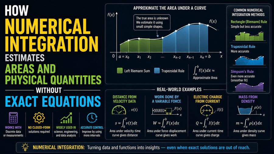
Many problems in mathematics, science, and engineering involve finding the total effect of something that changes continuously. We may want to calculate the area under a curve, the distance traveled by a vehicle whose speed changes every moment, the total energy consumed by a machine with varying power demand, or the amount of fluid flowing through a pipe over time.

In ideal textbook problems, these quantities can often be found using an exact mathematical integral. But real-world data is rarely so convenient. Measurements may come from sensors, experiments may produce only a table of values, or the underlying equation may be too complicated to integrate symbolically.

This is where numerical integration becomes extremely useful. 🔢📊

Numerical integration estimates the value of an integral using a finite set of calculations. Instead of requiring a perfect antiderivative, it divides a complicated area or accumulated quantity into smaller pieces and adds approximations of those pieces together.

The central idea is simple:

If an exact answer is difficult to calculate, approximate the whole by adding many small, manageable parts.

🧮 What Does Integration Actually Measure?

In calculus, integration is often introduced as a method for finding the area underneath a curve.

Suppose a function is written as:

y = f(x)

The definite integral

∫ₐᵇ f(x) dx

represents the accumulated value of the function between the limits a and b.

Geometrically, if the function stays above the horizontal axis, this can represent the area between the curve and the axis.

But integration is much more than an area-finding tool.

It can calculate:

• 🚗 distance from changing velocity,
• ⚡ energy from varying power,
• 💧 total flow from a changing flow rate,
• 🌡️ accumulated heat transfer,
• 🧱 mass from varying density,
• 📈 total probability from a probability density,
• 🔬 quantities derived from experimental measurements.

Integration converts a rate, density, or continuously varying quantity into a total.

❓ Why Can’t We Always Integrate Exactly?

Some mathematical functions have simple antiderivatives.

For example:

∫ x² dx = x³/3 + C

This can be evaluated exactly.

However, many practical problems do not have such convenient solutions.

A function may be:

• too complicated for elementary integration,
• generated by a computer simulation,
• measured experimentally rather than given by an equation,
• affected by noise,
• available only as a set of discrete points,
• impossible to integrate using standard symbolic formulas.

For example, imagine a temperature sensor records a machine’s power consumption every second:

Time (s)     Power (W)
0            120
1            138
2            151
3            147
4            160

There may be no exact equation describing the power between those measurements.

Yet engineers can still estimate the total energy consumed.

Numerical integration makes this possible. ⚙️

📦 The Basic Idea: Divide the Area Into Small Pieces

Imagine a curved line drawn above the x-axis.

Instead of finding the exact area underneath it, divide the interval into many small sections.

Each small section can be approximated by a simple shape such as:

• a rectangle,
• a trapezoid,
• a parabola-shaped segment.

The estimated areas of all these pieces are then added.

The smaller the pieces become, the more closely they can follow the original curve. 📏

This general principle is the foundation of most numerical integration methods.

🟦 The Rectangle Method

The simplest numerical integration technique approximates the area using rectangles.

Suppose the interval from a to b is divided into equal sections of width:

Δx

For each section, the function height is evaluated at a chosen point.

The approximate area of each rectangle is:

Area ≈ height × width

or:

Area ≈ f(x)Δx

The total estimated integral becomes the sum of all rectangle areas.

This approach is closely related to the idea behind Riemann sums.

⬅️ Left-Endpoint Method

The height of each rectangle is taken from the left side of the interval.

➡️ Right-Endpoint Method

The height is taken from the right side.

🎯 Midpoint Method

The function is evaluated at the middle of each interval.

The midpoint method is often more accurate than simply using left or right endpoints because it tends to balance errors more effectively.

🔺 The Trapezoidal Rule

A major improvement over basic rectangles is the trapezoidal rule.

Instead of assuming the function remains constant across each interval, the method connects two neighboring data points with a straight line.

The area underneath that line forms a trapezoid.

For points:

(x₀, y₀) and (x₁, y₁)

the approximate area is:

A ≈ (x₁ – x₀)(y₀ + y₁) / 2

In simpler terms:

Area = width × average height

This method often provides a better approximation because a sloping straight line usually follows a curved function more closely than a flat rectangle does. 📐

📊 Example of the Trapezoidal Rule

Suppose a vehicle’s speed is measured once every second:

Time (s)     Speed (m/s)
0            0
1            4
2            7
3            9

Distance is the integral of velocity with respect to time.

Between 0 and 1 second:

Distance ≈ 1 × (0 + 4)/2 = 2 m

Between 1 and 2 seconds:

Distance ≈ 1 × (4 + 7)/2 = 5.5 m

Between 2 and 3 seconds:

Distance ≈ 1 × (7 + 9)/2 = 8 m

Total estimated distance:

2 + 5.5 + 8 = 15.5 m

Even without knowing the exact velocity equation, numerical integration gives a useful estimate of the distance traveled. 🚗📏

🌀 Simpson’s Rule

For smoother curves, Simpson’s rule can provide even better accuracy.

Instead of connecting points with straight lines, Simpson’s rule approximates sections of the function using parabolic curves.

For two equal subintervals with three points:

x₀, x₁, x₂

the approximation is:

∫ f(x) dx ≈ h/3 [f(x₀) + 4f(x₁) + f(x₂)]

where h is the spacing between the points.

Notice the weights:

1, 4, 1

When Simpson’s rule is extended across more intervals, the pattern becomes:

1, 4, 2, 4, 2, 4, …, 1

Because parabolic curves can follow smooth functions more closely than straight lines, Simpson’s rule can achieve high accuracy with relatively few evaluation points. 🎯

⚡ Why Smaller Step Sizes Usually Improve Accuracy

Numerical integration involves approximation error.

If the interval is divided into only a few large sections, the simple shapes may not follow the original function very well.

If the interval is divided into many smaller sections, each approximation covers a smaller part of the curve.

For example:

Large intervals → rough estimate

Small intervals → finer estimate

This relationship is why reducing the step size often improves numerical accuracy.

However, smaller steps require more calculations.

Engineers therefore balance:

• accuracy,
• computation time,
• memory use,
• data availability.

Modern computers can often process millions of integration steps quickly, but very large simulations may still require careful optimization. 💻

🎯 What Is Integration Error?

Numerical integration does not usually produce an exact result.

The difference between the estimated value and the true integral is called the numerical error.

Error can come from several sources.

📏 Discretization Error

This occurs because a smooth curve is approximated using a finite number of pieces.

🔢 Rounding Error

Computers store numbers with finite precision.

Very large calculations can accumulate small rounding errors.

📡 Measurement Error

If the input data comes from sensors, the original measurements may already contain noise or uncertainty.

🧮 Model Error

The mathematical function itself may only approximate the physical system.

Numerical integration cannot make inaccurate input data magically exact.

The quality of the final result therefore depends on both the numerical method and the quality of the available data.

🔄 Adaptive Numerical Integration

Sometimes a function changes slowly in one region and rapidly in another.

Using the same step size everywhere may be inefficient.

Adaptive integration solves this problem by changing the step size automatically.

Where the function is smooth:

➡️ larger intervals can be used.

Where the function changes rapidly:

➡️ smaller intervals are used.

The algorithm repeatedly estimates the local error and subdivides difficult regions until the desired accuracy is reached. 🎯

This allows computational effort to be concentrated where it is most useful.

Adaptive algorithms are widely used in scientific software because they can provide high accuracy without unnecessarily evaluating the function everywhere.

🚗 Numerical Integration in Motion and Transportation

One of the clearest physical applications involves motion.

Velocity tells us how quickly position changes.

Therefore:

Distance = ∫ velocity dt

If a vehicle’s speedometer or GPS system provides velocity measurements over time, numerical integration can estimate the distance traveled.

Similarly:

Velocity = ∫ acceleration dt

An accelerometer in a smartphone, aircraft, robot, or navigation system can measure acceleration.

Integrating those measurements can estimate changes in velocity.

Integrating again can estimate changes in position. 📱✈️🤖

In practice, sensor noise causes errors to accumulate, so navigation systems often combine numerical integration with GPS and other measurements.

⚡ Calculating Energy From Power

Power represents the rate at which energy is transferred or consumed.

Therefore:

Energy = ∫ Power dt

Suppose a factory machine consumes varying amounts of electrical power throughout the day.

A monitoring system may record:

09:00 → 5.2 kW
09:01 → 5.7 kW
09:02 → 6.1 kW
09:03 → 5.8 kW

Numerical integration can use these measurements to estimate total energy consumption.

This principle is used in:

• smart meters,
• battery monitoring,
• industrial energy management,
• renewable-energy systems,
• electric vehicles. 🔋⚡

💧 Measuring Fluid Flow

Flow meters often report a flow rate, such as liters per second.

To find the total amount of liquid that passed through a pipe:

Total volume = ∫ flow rate dt

If the flow changes continuously, numerical integration can estimate total volume from periodic sensor measurements.

For example, a water-treatment plant may record flow every few seconds.

Adding the numerically integrated flow over several hours gives an estimate of total water processed. 💧🏭

The same idea is used in oil pipelines, chemical plants, medical infusion systems, and fuel-management systems.

🌡️ Heat Transfer and Thermal Engineering

Heat-transfer rates can vary as temperatures change.

If engineers know the rate of heat flow over time, the total transferred energy is:

Heat energy = ∫ heat-transfer rate dt

Numerical integration is therefore important in thermal simulations involving:

• engines,
• furnaces,
• heat exchangers,
• electronics cooling,
• buildings,
• batteries.

It can also be used to integrate temperature-dependent material properties across a range of operating conditions. 🌡️🔥

🧱 Calculating Mass From Varying Density

Suppose a material has nonuniform density.

The density may change depending on position.

Mass can be calculated by integrating density across the object’s volume:

Mass = ∫ density dV

For complicated shapes or measured density distributions, an exact symbolic calculation may be impossible.

Numerical integration divides the object into many small volume elements.

The mass of each element is estimated:

Small mass ≈ density × small volume

Then all the pieces are added together.

This principle appears in mechanical engineering, geophysics, material science, and structural analysis. 🪨🏗️

🏗️ Numerical Integration in Structural Engineering

Engineers often need to calculate quantities such as:

• bending moments,
• distributed loads,
• center of mass,
• deformation,
• stress energy.

Suppose a beam carries a load that varies irregularly along its length.

If the load distribution comes from experimental measurements rather than a neat formula, numerical integration can calculate the total force or moment.

This allows engineers to analyze real structures even when the loading is complicated. 🏢

📈 Numerical Integration in Probability

Probability theory also relies heavily on integration.

For a continuous probability distribution, probability corresponds to the area under a probability density function.

For example:

P(a ≤ X ≤ b) = ∫ₐᵇ f(x) dx

Some probability distributions have convenient analytical formulas.

Others require numerical integration.

Computer programs therefore use numerical techniques to evaluate probabilities in statistics, finance, engineering reliability, machine learning, and scientific research. 📊🎲

💰 Finance and Economics

Numerical integration appears in financial models where quantities vary continuously.

Applications may include:

• option pricing,
• accumulated interest models,
• expected values,
• risk calculations,
• economic growth models.

Complex financial models often involve probability distributions that cannot be integrated easily by hand.

Numerical methods allow analysts to estimate these quantities efficiently. 💹

🔬 Experimental Science

One of the greatest strengths of numerical integration is that it can work directly with measured data.

Suppose a scientist performs an experiment and records the intensity of a signal at different wavelengths.

The total signal intensity may correspond to the area underneath the measured curve.

There may be no known equation describing the curve.

But the trapezoidal rule can still estimate the total area using the data points themselves. 🔬📊

This makes numerical integration extremely valuable in laboratories.

💻 How Computers Perform Numerical Integration

Computers are particularly well suited to numerical integration because the procedure involves repeated calculations.

A program can:

1. choose a range,
2. divide it into intervals,
3. evaluate the function,
4. calculate approximate areas,
5. add them together,
6. estimate the remaining error.

For a complicated scientific model, this process may be repeated millions or billions of times.

High-performance computing systems can perform numerical integration over multidimensional spaces for simulations involving fluid mechanics, electromagnetism, quantum physics, climate science, and engineering design. 🖥️⚙️

🌐 What About Integrals With Many Dimensions?

Some problems require integration over two, three, or many dimensions.

For example, calculating a volume may involve a double integral:

∫∫ f(x,y) dx dy

A three-dimensional physical quantity may require a triple integral.

Numerical techniques can extend the same basic idea by dividing the region into small cells or elements.

However, as the number of dimensions increases, the number of required calculations can grow extremely quickly.

This challenge is sometimes called the curse of dimensionality.

For very high-dimensional problems, traditional grid-based integration may become impractical.

🎲 Monte Carlo Integration

One powerful method for high-dimensional problems is Monte Carlo integration.

Instead of dividing the entire space into a rigid grid, Monte Carlo methods use random sampling. 🎲

Imagine estimating the area of an irregular shape by randomly throwing thousands of points into a surrounding rectangle.

If 70% of the points land inside the shape, then approximately 70% of the rectangle’s area belongs to the shape.

The same statistical idea can estimate complicated multidimensional integrals.

Monte Carlo integration is widely used in:

• particle physics,
• financial modeling,
• radiation transport,
• statistical mechanics,
• computer graphics,
• uncertainty analysis.

Its accuracy improves as the number of random samples increases.

⚖️ Choosing the Right Integration Method

No single numerical method is best for every problem.

The rectangle method is simple but may require many intervals.

The trapezoidal rule works very well for tabulated data and is easy to implement.

Simpson’s rule is often highly accurate for smooth functions.

Adaptive methods concentrate calculations where the function is difficult.

Monte Carlo techniques can handle problems with many dimensions.

Engineers and scientists choose methods based on:

• data type,
• required accuracy,
• smoothness of the function,
• number of dimensions,
• available computing power,
• acceptable computation time.

The choice of algorithm can make an enormous difference in efficiency.

🧠 Why Numerical Integration Matters

Exact mathematical solutions are extremely valuable, but the physical world rarely follows perfectly convenient equations.

Real sensors produce discrete measurements.

Experiments produce tables.

Computer simulations generate numerical outputs.

Complex systems may involve equations whose antiderivatives cannot be written using familiar functions.

Numerical integration allows us to continue calculating useful physical quantities even in these situations. 🔢🌍

Instead of asking:

“Can we find the exact formula?”

numerical integration asks:

“Can we approximate the total accurately enough using the information we actually have?”

For many real-world engineering problems, that second question is far more useful.

📐 Turning Small Estimates Into Powerful Answers

Numerical integration is built on a remarkably simple strategy: divide a complicated total into manageable pieces, approximate each piece, and add them together.

Rectangles provide the simplest approach.

Trapezoids follow changing data more closely.

Simpson’s rule uses parabolic approximations for higher accuracy.

Adaptive techniques automatically refine difficult regions, while Monte Carlo integration helps tackle complex high-dimensional problems. 🎯

These methods allow computers to estimate quantities that would otherwise be extremely difficult—or impossible—to calculate exactly.

From determining the distance traveled by a changing-speed vehicle 🚗 to measuring energy consumption ⚡, fluid volume 💧, probability 📊, heat transfer 🔥, and experimental signal strength 🔬, numerical integration turns scattered measurements and complex functions into meaningful totals.

Its central principle can be summarized simply:

When an exact integral is unavailable, many carefully calculated small approximations can combine to produce a remarkably accurate estimate of the whole. 📐➕🔢➡️🎯