📐 How Runge–Kutta Methods Predict the Behavior of Dynamic Engineering Systems

Engineering systems rarely remain perfectly static. A vehicle accelerates and slows down, a suspension vibrates after hitting a bump, an electrical current changes after a switch closes, a chemical reactor heats up, and a spacecraft continuously changes position and velocity as gravitational forces act on it. 🚗⚡🛰️

To predict how these systems behave over time, engineers often describe them using differential equations. These equations connect a system’s current state with its rate of change.

The challenge is that many real engineering differential equations cannot be solved easily with a neat analytical formula. Even when an exact solution exists in theory, the model may be too complicated to solve symbolically once nonlinear forces, feedback controllers, temperature-dependent properties, aerodynamic effects, or multiple interacting components are included.

This is where Runge–Kutta methods become extremely valuable. 🧮

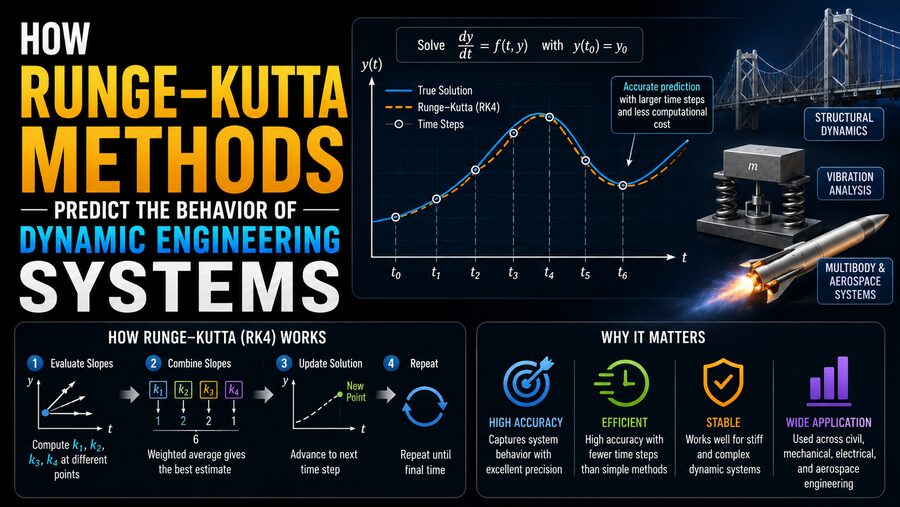
Runge–Kutta methods are numerical techniques that approximate the future state of a dynamic system by evaluating its rate of change at several carefully chosen points within each time step. Among them, the fourth-order Runge–Kutta method, usually called RK4, has become one of the best-known numerical integration techniques in engineering and science.

It provides a powerful compromise between simplicity, computational cost, and accuracy.

🔍 What Is a Dynamic Engineering System?

A dynamic system is one whose condition changes with time.

Engineers often describe the condition of such a system using state variables.

For a moving vehicle, state variables might include:

Position
Velocity
Acceleration-related quantities

For an electrical circuit, they might include:

Capacitor voltage
Inductor current

For a thermal system:

Temperature
Heat flow

For an aircraft:

Position
Velocity
Pitch angle
Roll angle
Yaw angle
Angular rates

The mathematical model describes how these variables change.

A simple differential equation might be written as:

dy/dt = f(t, y)

This means that the rate of change of y depends on time t, the current value of y, or both.

If engineers know the current state and the governing equation, they want to answer an important question:

What will the state be a short time later? ⏱️

Runge–Kutta methods provide one way to estimate that answer.

📈 Why Differential Equations Matter in Engineering

Differential equations appear almost everywhere in engineering because physical laws often describe rates of change.

Newton’s second law states:

F = ma

Since acceleration is the rate of change of velocity, and velocity is the rate of change of position, mechanical motion naturally produces differential equations.

Electrical circuits provide another example.

For a capacitor:

i = C dv/dt

For an inductor:

v = L di/dt

These relationships describe how voltage and current evolve over time. ⚡

Heat transfer, fluid flow, control systems, chemical kinetics, population models, and structural vibration also involve differential equations.

The equations may be straightforward to write but difficult to solve exactly.

🧮 The Simplest Numerical Idea: Euler’s Method

Before understanding Runge–Kutta methods, it helps to look at a simpler numerical technique called Euler’s method.

Suppose we know the current value:

yₙ

at time:

tₙ

and we want to estimate the value after a small time step h.

Euler’s method calculates the current slope:

f(tₙ, yₙ)

and assumes that slope remains constant across the entire time step.

The estimate becomes:

yₙ₊₁ = yₙ + h f(tₙ, yₙ)

Conceptually:

new value = old value + time step × current rate of change

This approach is intuitive and easy to calculate.

Unfortunately, it can also be inaccurate. ⚠️

🛣️ Why Euler’s Method Can Drift Away From Reality

Imagine walking along a curved road.

At your starting location, you determine the direction in which the road is pointing.

Euler’s method essentially says:

“Follow that direction in a straight line until the next step.”

But if the road curves significantly during the step, your straight-line prediction will miss the actual path.

Taking very small steps can reduce the error, but this requires many more calculations.

Runge–Kutta methods improve the prediction by checking the slope at additional locations within the step. 🛣️

Instead of trusting only the slope at the beginning, they ask:

How is the slope changing as we move forward?

🚀 The Basic Idea Behind Runge–Kutta Methods

A Runge–Kutta method evaluates the differential equation multiple times during one step.

Each evaluation provides an estimate of the local slope.

These slopes are then combined using carefully chosen weights.

The result is a much better estimate of how the system changes across the entire step.

Different Runge–Kutta methods use different numbers of slope evaluations.

The most famous is RK4, which uses four.

4️⃣ Understanding the Fourth-Order Runge–Kutta Method

For the differential equation:

dy/dt = f(t, y)

RK4 calculates four quantities commonly called:

k₁, k₂, k₃, k₄

They represent slope estimates at different points in the time interval.

1️⃣ First Slope: k₁

The first slope is evaluated at the beginning:

k₁ = f(tₙ, yₙ)

This is essentially the same initial slope used by Euler’s method.

It asks:

How quickly is the system changing right now?

2️⃣ Second Slope: k₂

RK4 then moves approximately halfway through the time step using the first slope:

k₂ = f(tₙ + h/2, yₙ + hk₁/2)

This asks:

If the system follows the initial trend halfway forward, what would the slope be there?

3️⃣ Third Slope: k₃

Another midpoint estimate is calculated:

k₃ = f(tₙ + h/2, yₙ + hk₂/2)

This midpoint is based on the improved k₂ estimate.

4️⃣ Fourth Slope: k₄

Finally, RK4 estimates the slope at the end of the time step:

k₄ = f(tₙ + h, yₙ + hk₃)

The method has now examined the beginning, two midpoint estimates, and the end.

⚖️ Combining the Four Slopes

RK4 combines these slopes as:

yₙ₊₁ = yₙ + h(k₁ + 2k₂ + 2k₃ + k₄)/6

Notice the weighting:

k₁ gets weight 1
k₂ gets weight 2
k₃ gets weight 2
k₄ gets weight 1

The midpoint slopes receive extra influence because they provide particularly useful information about how the system behaves throughout the interval.

This weighted combination provides a remarkably accurate estimate for many smooth dynamic systems. 🎯

🚗 Example: Predicting Vehicle Motion

Imagine an engineer modeling a car accelerating under engine force while aerodynamic drag opposes its motion.

A simplified equation might be:

m dv/dt = Fengine - Fdrag

Aerodynamic drag often depends approximately on the square of velocity:

Fdrag = ½ρCdAv²

Therefore:

dv/dt = (Fengine - ½ρCdAv²) / m

This equation is nonlinear because velocity appears squared.

An RK4 simulation can estimate the car’s velocity over time.

At every time step, the algorithm evaluates acceleration several times using slightly different predicted velocities.

It then combines those estimates to calculate a new velocity.

Repeating the process might produce predictions such as:

Velocity after 1 second
Velocity after 5 seconds
Time required to reach 100 km/h
Maximum speed when drag balances engine force

🚗💨

The same model could also integrate velocity to estimate vehicle position.

🏗️ Predicting Structural Vibrations

Mechanical and civil engineers frequently study vibrations.

Consider a mass attached to a spring and damper.

Its equation of motion might be:

m d²x/dt² + c dx/dt + kx = F(t)

where:

m = mass
c = damping coefficient
k = spring stiffness
x = displacement
F(t) = external force

This is a second-order differential equation.

Runge–Kutta methods are commonly designed around first-order systems, so engineers rewrite it using state variables.

Let:

x₁ = x

and:

x₂ = dx/dt

Then:

dx₁/dt = x₂

and:

dx₂/dt = [F(t) - cx₂ - kx₁] / m

Now RK4 can integrate both state variables simultaneously.

The simulation can predict how a structure vibrates after an impact or under periodic loading. 🏢

⚡ Electrical Circuit Simulation

Runge–Kutta methods can also simulate electrical systems.

Consider a simple resistor-capacitor circuit.

A capacitor charging through a resistor can be modeled by:

dV/dt = (Vs - V) / RC

where:

V = capacitor voltage
Vs = source voltage
R = resistance
C = capacitance

RK4 can predict how capacitor voltage rises with time.

For more complicated circuits containing nonlinear devices, switches, inductors, and controllers, numerical integration becomes even more useful.

Circuit-simulation software often relies on numerical integration techniques, although professional simulators may select specialized methods depending on stability requirements. 🔌

🛰️ Simulating Spacecraft Motion

Orbital mechanics provides another dramatic example.

The gravitational force acting on a spacecraft changes continuously as its position changes.

For a simplified two-body problem:

d²r/dt² = -μr/|r|³

The spacecraft’s acceleration depends on its current position.

Engineers can convert the equations into first-order position and velocity equations and integrate them numerically.

A Runge–Kutta solver can then calculate:

Position
Velocity
Orbital trajectory
Maneuver response
Re-entry paths

over many successive time steps. 🛰️🌍

For high-precision aerospace applications, more advanced adaptive or specialized integrators may be used, but Runge–Kutta methods remain foundational.

🤖 Runge–Kutta Methods in Control Systems

Control engineers frequently simulate dynamic systems before implementing controllers on real equipment.

Imagine designing a controller for a drone.

Its mathematical model may describe:

Position
Linear velocity
Angular orientation
Angular velocity
Motor thrust
Aerodynamic forces

The controller continuously generates motor commands based on predicted system behavior.

Numerical integration allows engineers to simulate how the drone responds to those commands.

They can test:

Stability
Disturbance rejection
Overshoot
Settling time
Controller tuning

without risking physical hardware during every experiment. 🚁

🌡️ Thermal Engineering Applications

Temperature also changes dynamically.

A simplified thermal system could follow:

mc dT/dt = Qin - Qout

where:

m = mass
c = specific heat capacity
T = temperature
Qin = incoming heat rate
Qout = outgoing heat rate

If heat loss depends on temperature, the equation changes continuously as the object warms or cools.

Runge–Kutta integration can predict temperature histories in:

Batteries 🔋
Engines
Electronic components
Furnaces
Buildings
Heat exchangers

This can help engineers prevent overheating and optimize energy use.

🧪 Chemical Reactor Modeling

Chemical reaction rates often depend strongly on concentrations and temperature.

Suppose reactant A converts into product B.

A simple reaction model might be:

dCA/dt = -kCA

More complex reactors may contain several simultaneous reactions:

dCA/dt = f₁(CA, CB, T)

dCB/dt = f₂(CA, CB, T)

dT/dt = f₃(CA, CB, T)

These equations are coupled, meaning each variable can affect the others.

Runge–Kutta methods can integrate the entire system together and predict concentration and temperature over time. 🧪🔥

🔗 Solving Multiple Equations at Once

Real engineering models rarely contain just one variable.

Suppose a system has state vector:

x = [x₁, x₂, x₃, ..., xₙ]

The equations may be written compactly as:

dx/dt = f(t, x)

Each RK4 slope then becomes a vector rather than a single number.

For example:

k₁ = f(tₙ, xₙ)

The remaining stages are calculated in the same general way.

This means the method can simulate systems with many interacting states.

A vehicle model might include dozens of variables. An aircraft model might include even more.

The underlying RK4 principle remains unchanged. 🧠

🎯 Why RK4 Is So Accurate

RK4 is called a fourth-order method because of the way its numerical error decreases as the step size becomes smaller.

For sufficiently smooth problems, the accumulated global error scales approximately with:

h⁴

where h is the time-step size.

If the time step is reduced, the error can decrease very rapidly.

This makes RK4 considerably more accurate than simple Euler integration for the same step size in many ordinary problems.

However, accuracy always depends on the characteristics of the system and the chosen time step.

⏱️ Why Time-Step Size Matters

Even a good numerical method can give poor results if the time step is too large.

Imagine simulating a vibration that oscillates 100 times per second but using one integration step every second.

The solver would completely miss most of the motion.

A smaller time step captures faster system dynamics more accurately.

However, smaller steps require more computations.

Engineers therefore balance:

Accuracy ↔ Computational cost

This tradeoff is one of the central concerns in numerical simulation. ⚖️

🔄 Adaptive Runge–Kutta Methods

Instead of using the same step size everywhere, many modern solvers use adaptive step sizing.

The basic idea is:

Use small steps when the solution changes rapidly.
Use larger steps when the solution changes smoothly.

This can significantly improve efficiency.

Popular adaptive Runge–Kutta approaches estimate their own local error by calculating solutions of two different orders.

For example, a method might produce both a fourth-order and fifth-order estimate.

The difference between them provides information about numerical error.

If the error is too large:

Reduce the step size.

If the error is comfortably small:

Increase the step size.

This allows the solver to automatically concentrate computing effort where it is most needed. 🤖

📉 Local Error vs. Global Error

Numerical integration introduces approximation error.

Two important concepts are:

🔹 Local Truncation Error

This is the error introduced during a single integration step, assuming the starting point is exact.

🔸 Global Error

This is the accumulated difference between the numerical solution and the true solution after many steps.

A numerical method that performs well over one step can still accumulate error during a long simulation.

This is why engineers evaluate not only theoretical order but also stability, time-step size, and long-term behavior.

⚠️ Numerical Stability

Accuracy is not the only issue.

A numerical method must also remain stable.

Some dynamic systems contain processes occurring on dramatically different time scales.

For example, one electrical phenomenon may occur in microseconds while another evolves over seconds.

Such systems can be stiff.

Explicit Runge–Kutta methods such as classical RK4 may require extremely small time steps for stiff systems, even if the slowly changing part of the solution appears simple.

In these situations, engineers often use specialized implicit numerical methods designed for stiff differential equations.

So RK4 is powerful, but it is not universally the best solver. 🛠️

🆚 RK4 vs. Euler’s Method

Euler’s method requires one main slope evaluation per step.

RK4 requires four.

So RK4 performs more work during each step.

However, it often achieves much greater accuracy.

Euler:

Very simple
Computationally inexpensive per step
Useful for teaching and rough simulations
Often requires small steps

RK4:

More calculations per step
Much better accuracy for many smooth problems
Widely useful in engineering simulation
Still relatively straightforward to implement

For many applications, the additional slope evaluations are worth the improvement in accuracy. 📊

💻 Runge–Kutta Methods in Engineering Software

Engineers often encounter numerical integration inside software without manually calculating every RK stage.

Simulation environments can automatically integrate differential equations representing:

Mechanical systems
Electrical systems
Control systems
Thermal models
Fluid systems
Biological systems
Aerospace vehicles

Numerical solver libraries also provide Runge–Kutta algorithms in programming languages such as Python, MATLAB, C++, Julia, and others.

When engineers select a numerical solver, they may choose between:

Fixed-step methods
Adaptive-step methods
Explicit methods
Implicit methods
Specialized stiff-system solvers

Understanding Runge–Kutta theory helps engineers make sensible solver choices rather than treating simulation software as a mysterious black box. 🖥️

🏎️ Real-Time Simulation

Some engineering simulations must operate in real time.

Examples include:

Driving simulators
Flight simulators
Hardware-in-the-loop testing
Robotics
Embedded control systems

In these applications, the numerical integration must finish before the next real-time update is required.

A solver that is extremely accurate but computationally expensive may not be practical.

Fixed-step Runge–Kutta methods can be attractive because their computational workload is predictable.

Engineers select a time step that balances real-time constraints with acceptable numerical accuracy. ⏲️

🔬 Model Accuracy vs. Solver Accuracy

A crucial engineering lesson is that a very accurate numerical solver cannot compensate for an incorrect physical model.

Suppose an aerodynamic simulation ignores a major drag force.

Even if RK4 integrates the equations with extraordinary numerical precision, the result can still be physically wrong.

There are therefore two separate questions:

Does the mathematical model represent reality well?
Does the numerical solver accurately integrate that model?

Both matter.

Numerical methods solve equations; they do not automatically make those equations correct. 🎯

🧩 A Simple Intuitive Analogy

Imagine predicting the path of a cyclist traveling along a winding road.

Euler’s method checks the cyclist’s direction only at the beginning of each interval and predicts forward.

RK4 behaves more like an observer who checks:

The direction at the start
An estimated direction halfway through
Another refined midpoint direction
The direction near the end

It then combines all four observations to estimate where the cyclist should actually finish the interval.

🚴➡️

By sampling how the direction changes throughout the step, RK4 follows curves much more accurately than a method relying only on the initial direction.

🌍 Where Runge–Kutta Methods Are Used

Runge–Kutta techniques appear throughout engineering and scientific computing.

Applications include:

Vehicle dynamics 🚗
Aircraft simulation ✈️
Spacecraft trajectories 🛰️
Robotics 🤖
Electrical circuits ⚡
Control systems
Structural vibration 🏗️
Heat-transfer analysis 🌡️
Chemical reactors 🧪
Fluid systems
Biological models
Energy systems
Battery modeling 🔋

Whenever engineers need to predict a continuously changing system governed by differential equations, numerical integration methods are likely involved.

✅ Conclusion

Runge–Kutta methods help engineers predict dynamic behavior by converting differential equations into a sequence of manageable numerical calculations.

Instead of trying to find an exact mathematical expression for the entire future of a system, the solver moves forward one small time interval at a time. ⏱️

The classical fourth-order Runge–Kutta method improves accuracy by evaluating the system’s rate of change four times during each step. It checks the slope at the beginning, examines two estimates near the midpoint, evaluates another near the end, and combines them using carefully designed weights.

This approach allows RK4 to follow curved and nonlinear behavior far more accurately than a simple single-slope method such as Euler integration.

From predicting how a suspension vibrates after a road impact to simulating a spacecraft orbit, an electrical circuit, a chemical reactor, or a robotic controller, Runge–Kutta techniques provide engineers with a practical way to turn mathematical models into predictions. 📐⚙️

More advanced versions can automatically change their time-step size, spending extra computation when the system changes quickly and larger steps when behavior is smooth.

Runge–Kutta methods are not perfect. Very stiff systems may require different numerical techniques, and every simulation still depends on the quality of its physical model.

But their combination of accuracy, versatility, and conceptual simplicity has made them some of the most important tools in numerical engineering.

Whenever a computer simulation shows how a complex system will evolve second by second, there is a good chance that somewhere underneath the graphics, a numerical integration algorithm is repeatedly asking one fundamental question:

Given how the system is changing right now, where will it be next? 🧮🚀