
A pump test ends with a spreadsheet full of readings: flow rate, pressure rise, motor current, fluid temperature, and vibration. The immediate question is rarely just “what happened?” More often, it is “what will happen at the next operating condition?”
Engineers make these predictions constantly. They estimate deflection from load, energy use from production rate, temperature from time, or material strength from composition. A good estimate supports design choices, maintenance planning, and sensible experiments.
Linear regression is one of the most useful starting tools for turning measured data into a prediction. It is mathematically approachable, easy to implement, and surprisingly powerful when its assumptions match the problem.
Its apparent simplicity can also be misleading. A line fitted to numbers is not automatically a trustworthy engineering model. The quality of the measurement system, the physics, the operating range, and the way uncertainty is handled all determine whether a prediction deserves confidence.
📈 What Linear Regression Does
Linear regression describes the relationship between an output, called the response or dependent variable, and one or more inputs, called predictors or independent variables. It fits a mathematical relationship that can estimate the response for new input values.
In simple linear regression, the relationship is a straight line:
y = b₀ + b₁x + εHere, y is the measured output, x is the input, b₀ is the intercept, b₁ is the slope, and ε represents the part not explained by the line. The fitted equation omits the unknown error term and is written as ŷ = b₀ + b₁x.
🧭 Why Engineers Use It
Regression converts scattered observations into a compact model. Rather than reviewing hundreds of test points each time a decision is needed, an engineer can use a validated equation to estimate a likely value and its uncertainty.
Common uses include calibration curves for instruments, preliminary design estimates, process monitoring, test-data reduction, and empirical correlations. It is especially helpful when theory suggests the variables should be related but real equipment introduces friction, tolerances, heat loss, or other effects that are difficult to model exactly.
A regression model is not a replacement for engineering mechanics, thermodynamics, or materials science. It is a practical complement: physics guides what to measure and what form of relationship is plausible; regression estimates that relationship from data.
🔧 A Simple Engineering Example
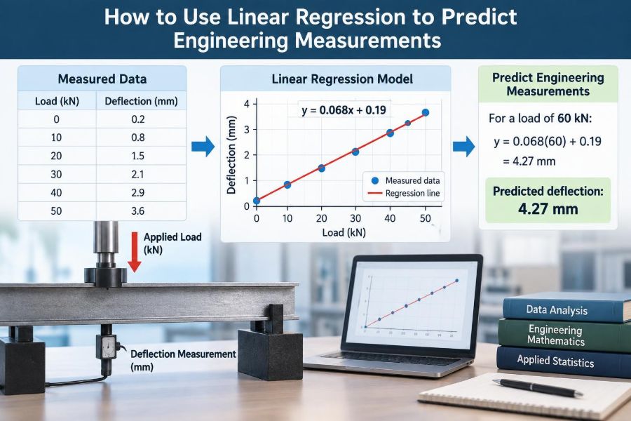
Suppose a laboratory applies increasing tensile loads to a bracket and measures tip deflection. Over a modest elastic range, the data may show that deflection rises nearly proportionally with load.
A fitted result such as deflection = 0.12 + 0.0048 × load might use millimetres for deflection and newtons for load. The slope says the fitted model predicts about 0.0048 mm more deflection per additional newton within the tested range.
The intercept of 0.12 mm deserves investigation. It could reflect fixture settling, sensor zero offset, initial clearance, or simply random fitting variation. An intercept is a fitted parameter, not automatically a physical constant.
🎯 Define the Prediction Question First
Before calculating anything, state exactly what must be predicted. “Predict performance” is too broad. “Estimate pressure drop across this filter at a specified flow rate and fluid temperature” is a usable prediction question.
Define the output, relevant inputs, units, operating range, intended accuracy, and decision that will use the estimate. A model used to flag a possible process drift can tolerate more uncertainty than one used to set a structural load limit.
This framing also prevents an easy error: fitting every available spreadsheet column because it exists. Variables should enter the model because they have a plausible relationship to the response or a demonstrated predictive contribution.
📏 Choose a Measurable Response Variable
The response variable should match the engineering decision. If the concern is thermal expansion, the response might be final displacement. If the concern is manufacturing throughput, it might be cycle time or parts completed per hour.
Use a precise measurement definition. “Temperature” could mean inlet temperature, wall temperature, bulk fluid temperature, or a peak value over time. Mixing definitions creates noise that no statistical method can repair.
Record units alongside the data. Unit errors can produce a line that appears mathematically valid but is operationally useless. Consistent units also make slope interpretation much clearer.
🧩 Select Predictors With Physical Sense
For a first model, start with inputs that engineering reasoning identifies as likely drivers. Flow rate is a sensible predictor for pressure loss; applied load is sensible for elastic deflection; ambient temperature may be sensible for cooling-system demand.
Some relevant variables are not directly controllable but should still be recorded. For example, a machine’s output may depend on humidity, tool wear, operator setup, or batch material. Ignoring a major driver can make a model look unstable when the process, not the mathematics, is changing.
Conversely, adding weak or redundant predictors can make coefficients hard to interpret and may make predictions less reliable on new data.
🗂️ Build a Fit-for-Purpose Dataset
A useful dataset represents the conditions where predictions will be made. If a heat-exchanger model is trained only at low flow rates, it has not been tested as a high-flow model, even if its equation can generate a number there.
Plan measurements across the operating range rather than collecting many repeats at one convenient setting. Replicates are still valuable: they reveal repeatability and help separate genuine trends from measurement variation.
- Capture input settings and measured outputs.
- Record units, sensor identity, timestamps, and relevant operating conditions.
- Note adjustments, interruptions, and unusual events during testing.
- Preserve raw data separately from cleaned analysis data.
Good data records allow another engineer to understand why a result was obtained and whether the model applies to a new case.
🧪 Check Measurement Quality Before Modeling
Regression treats recorded values as data, not as unquestionable truth. A drifting thermocouple, saturated load cell, loose pressure tap, or transcription error can dominate the fitted line.
Check instrument calibration status, resolution, sampling procedure, and the time needed for the system to reach steady state. For dynamic systems, readings taken before settling may reflect transient behaviour rather than the intended operating relationship.
When the predictor itself has substantial measurement error, ordinary least squares can bias the estimated slope. In such cases, better instrumentation, repeated measurements, or specialized errors-in-variables methods may be more appropriate.
👀 Start With a Scatter Plot
Plot the response against each important predictor before fitting a model. A scatter plot often reveals curvature, separate operating regimes, outliers, recording mistakes, or changing variability that a summary table conceals.
For one input and one output, place the predictor on the horizontal axis and response on the vertical axis. Add units, identify test groups where useful, and avoid axes that hide meaningful variation.
Do not expect real engineering points to sit perfectly on a line. The useful question is whether the main pattern is reasonably linear over the relevant range and whether the remaining deviations behave sensibly.
📐 Understand the Least-Squares Fit
Ordinary least squares chooses the intercept and slope that make the total squared vertical differences between observed values and fitted values as small as possible. Those vertical differences are called residuals.
For observation i, the residual is:
eᵢ = yᵢ − ŷᵢSquaring makes positive and negative discrepancies contribute equally and gives larger discrepancies more influence. This is useful when errors are roughly well behaved, but it also means one extreme bad reading can pull a line noticeably.
🧮 Calculate the Simple Regression Equation
For hand calculation or a spreadsheet check, the slope and intercept can be obtained from:
b₁ = Σ[(xᵢ − x̄)(yᵢ − ȳ)] / Σ[(xᵢ − x̄)²]
b₀ = ȳ − b₁x̄
The bars denote sample means. Most engineering work will use spreadsheet functions, statistical software, or code, but understanding these expressions is useful: the slope comes from how input and output vary together relative to the spread in the input.
Never round coefficients aggressively during analysis. Retain adequate precision in the calculation and round the reported prediction only to a precision justified by the measurements.
🧠 Interpret the Slope in Engineering Units
The slope has units of “response units per predictor unit.” If pressure drop is in kilopascals and flow rate is in litres per minute, a slope of 1.6 means the fitted pressure drop increases by 1.6 kPa for each additional L/min.
This interpretation makes slopes useful for sensitivity discussions. A steep slope means small input changes may matter greatly. A shallow slope may mean the input has little practical influence across the observed range, even if a statistical test labels it detectable.
Always ask whether the direction and size of the coefficient are physically credible. A surprising sign can reveal confounding, a wiring error, an omitted variable, or a genuinely interesting process effect that needs investigation.
🏁 Treat the Intercept Carefully
The intercept is the fitted response when all predictors equal zero. Sometimes zero is meaningful, such as zero applied load. Sometimes it is not, such as zero absolute operating pressure for equipment never used near that condition.
Do not claim the intercept describes a real system state merely because the equation includes it. If zero lies outside the data range, the intercept may be only a mathematical anchor for the line.
Forcing a regression through the origin should be based on physics and measurement design, not on a desire for a neat-looking equation. A forced-zero model can distort the slope if an offset is actually present.
🧱 Move to Multiple Linear Regression
Many engineering outputs depend on more than one input. Multiple linear regression extends the model:
ŷ = b₀ + b₁x₁ + b₂x₂ + ... + bₚxₚA pump’s power demand, for example, may be modeled from flow rate, pressure rise, and fluid temperature. A manufacturing cycle-time model may include part size, material grade, and machine setting.
Each coefficient is interpreted with the other included predictors held constant. That qualification matters. It is not simply the observed one-variable relationship when the predictors themselves move together.
🔄 Watch for Correlated Predictors
Predictors are correlated when they tend to change together. In a production line, feed rate and motor current may rise together; in weather-exposed equipment, ambient temperature and solar load may be linked.
Strong correlation between predictors, often called multicollinearity, can make individual coefficients unstable. The model may predict reasonably well while being unable to assign a reliable separate effect to each correlated input.
Inspect predictor plots and correlation measures, then use engineering judgement. Possible responses include removing a redundant variable, combining variables meaningfully, collecting a better-designed dataset, or accepting that the model is predictive rather than explanatory.
🧷 Include Categorical Operating Conditions
Not every useful predictor is numeric. Material grade, machine line, fixture type, or shift can be represented with indicator variables, often called dummy variables.
For example, a model can include a variable that is 0 for one fixture and 1 for another. Its coefficient estimates the fitted difference associated with the second fixture after accounting for other predictors.
Choose a clear reference category and ensure each category has enough observations. A category represented by only a few unusual tests may produce a coefficient that is more anecdotal than dependable.
🪜 Model Interactions When Effects Depend on Each Other
An interaction means the effect of one predictor changes with another. For example, increasing flow rate may affect pressure loss differently at different fluid viscosities.
A simple interaction term multiplies two predictors:
ŷ = b₀ + b₁(flow) + b₂(viscosity) + b₃(flow × viscosity)Interactions should have a physical rationale or clear pattern in the data. Adding many possible interactions without enough data quickly creates a complicated model that fits accidental fluctuations.
🌊 Recognize When a Straight Line Is Not Enough
Some engineering relationships are nonlinear by nature. Turbulent-flow pressure losses, heat-transfer effects, chemical rates, and material behaviour near failure may curve substantially over their working ranges.
A line can still be useful over a narrow local range. Outside that range, it may systematically overpredict or underpredict. A curved residual pattern is a warning that the chosen form misses structure.
Possible alternatives include a physically derived model, a transformed-variable model, a polynomial term used cautiously, piecewise regression for known regimes, or another regression method. The simplest adequate model is usually preferable to the most flexible one.
🪞 Use Residual Plots as a Diagnostic Tool
A residual plot shows residuals against fitted values, time, or a predictor. For a suitable linear model, residuals should appear as an unstructured cloud around zero rather than as an obvious curve, funnel, or sequence.
| Residual pattern | Possible interpretation | Useful response |
|---|---|---|
| Curved band | Missing nonlinear relationship | Reconsider model form or operating regimes |
| Funnel-shaped spread | Error variability changes with level | Consider transformation or weighted methods |
| Long runs above or below zero | Time dependence or process drift | Include time effects or revise sampling |
| One isolated extreme point | Outlier, special event, or data error | Investigate the original observation |
Diagnostics do not mechanically prove a model right or wrong. They help locate assumptions that deserve engineering investigation.
⏱️ Account for Time and Process Drift
Measurements taken in time order are often not independent. Tool wear, warming equipment, sensor drift, changing feedstock, or operator adjustments can make neighbouring readings more similar than distant readings.
If time is relevant, plot residuals in collection order. A steady rise or fall can indicate that the model is missing a changing condition. Randomly mixing test settings during data collection can reduce the risk that time trends are confused with an input effect.
For strongly time-dependent systems, ordinary regression may need augmentation with time-series or dynamic modeling methods. A static line cannot fully describe a system with memory.
🚩 Investigate Outliers Instead of Deleting Them
An outlier is a point that differs markedly from the pattern of most observations. It may be caused by a mistyped unit, a faulty sensor, a setup error, an unusual but real event, or a process condition not represented elsewhere.
Deleting points simply because they spoil the fit is poor practice. Return to test notes, raw instrument records, calibration information, and physical evidence. If an error is confirmed, correct or exclude it transparently; if it is real, it may reveal a limitation or failure mode worth understanding.
Also distinguish an outlier in the response from a high-leverage point with an unusual predictor value. A high-leverage point can strongly influence the line even when its residual is small.
📊 Do Not Rely on R-Squared Alone
R-squared describes the fraction of variation in the response that the fitted model accounts for within the dataset. A higher value often indicates a closer in-sample fit, but it is not a universal quality score.
A high R-squared can coexist with biased residuals, extrapolation risk, data leakage, or poor performance on future measurements. It can also rise merely because unnecessary predictors are added.
Use it alongside residual checks, engineering plausibility, prediction error measures, and validation on data not used to fit the model. For multiple regression, adjusted R-squared can be more informative than ordinary R-squared when comparing models with different numbers of predictors.
🎯 Separate Fit Quality From Prediction Accuracy
A model can describe the average trend well yet still have individual predictions that vary widely. Engineering decisions usually need this second question answered: how far might a future measurement fall from the predicted value?
Report a point prediction with an appropriate prediction interval when uncertainty matters. A prediction interval is wider than an interval for the mean response because it includes both uncertainty in the fitted line and ordinary variation among future observations.
The exact calculation depends on the regression assumptions and software method. More fundamentally, the interval is meaningful only for conditions similar to those represented by the data.
🧪 Validate With Unused Data
Validation checks whether a model works beyond the records used to create it. The cleanest approach is to reserve a representative set of measurements for testing, fit the model on the remaining data, and compare predictions with the held-out observations.
When data are limited, cross-validation repeatedly fits on subsets and evaluates on excluded subsets. For data with time order, keep the order in mind: testing a model on earlier records after training on later records may not reflect real deployment.
Compare errors in engineering units. A model with a modest-looking statistical error may still be unacceptable if its typical deviation is larger than the allowable process tolerance.
🗺️ Stay Inside the Supported Range
Interpolation estimates between observed input values. Extrapolation estimates beyond them. Interpolation is generally safer because the model is being used where its trend has been observed.
Extrapolation is risky because real systems often change regime: a material yields, a valve approaches a limit, a motor heats up, or a flow becomes turbulent. A straight line has no way to recognize such boundaries on its own.
Always state the validated range beside the equation. A useful model description says more than “use this formula”; it says which equipment, units, conditions, and input limits the formula represents.
🛠️ Build the Model in a Spreadsheet or Code
A spreadsheet is often sufficient for small, transparent analyses. Use a scatter plot, a regression tool or function, and residual columns. Keep formulas visible so that another reviewer can trace the calculation.
Statistical software and programming tools become especially useful for multiple predictors, diagnostic plots, automated validation, reproducible reports, and version-controlled workflows. The software does not choose the right variables or operating assumptions; it only performs calculations consistently.
A practical workflow is:
- Import and preserve raw measurements.
- Check units, missing values, and obvious recording errors.
- Plot the data and define a physically defensible model.
- Fit the model and inspect residuals.
- Validate predictions and document the supported range.
📝 Report an Equation So Others Can Use It
A regression result should be reproducible, not just a coefficient table pasted into a report. Include the response definition, predictor definitions, units, data source, sample range, fitting method, and relevant diagnostics.
State the equation with enough significant figures for use, but not so many that it implies impossible measurement precision. Explain whether the model is intended for prediction, calibration, screening, or interpretation.
For decisions with safety, quality, or regulatory consequences, document uncertainty, review requirements, and the action to take when an input is outside the model range. A model is part of a decision process, not a substitute for it.
⚠️ Avoid Common Regression Mistakes
Several errors recur in otherwise careful engineering analyses:
- Using an equation outside the measured operating range.
- Confusing correlation with a proven causal mechanism.
- Fitting a line without plotting raw data and residuals.
- Ignoring units, sensor offsets, or data collected during transients.
- Adding predictors until the in-sample fit looks impressive.
- Reporting a point estimate without considering uncertainty.
- Using a model trained on one machine, material batch, or environment as though it applies everywhere.
These are not merely statistical issues. Each one can lead to incorrect engineering action when the model is treated as more general than the evidence supports.
🔍 Distinguish Association From Causation
Regression identifies patterns of association in the supplied data. It does not by itself establish that changing a predictor will cause the estimated change in the response.
For example, motor current and product temperature may correlate because both increase with production rate. A regression coefficient for current does not prove that changing current independently changes temperature in the same way.
Causal claims require process knowledge and, where practical, controlled experiments or carefully designed observational studies. This distinction is crucial when a regression result will influence changes to an operating process.
⚖️ Know When Linear Regression Is the Right Tool
Linear regression is a strong choice when the response is continuous, the expected relationship is approximately linear over the target range, measurements are reasonably reliable, and the dataset represents future operating conditions.
It may be a poor choice when the output is a category, the relationship has abrupt thresholds, data are dominated by repeated time dependence, or important physical constraints are ignored. Other methods may be more appropriate, but a simpler linear baseline remains valuable for comparison.
Even when a more advanced model eventually wins, linear regression often exposes the core drivers, data-quality problems, and limits of predictability faster than a black-box approach.
🧱 A Practical Checklist Before Deployment
Before relying on a regression prediction, ask a short set of disciplined questions:
- Does the intended case match the equipment and operating conditions in the dataset?
- Are all inputs within the validated range and expressed in the correct units?
- Do residual diagnostics show a major unmodeled pattern?
- Has performance been checked on independent or held-out data?
- Is the prediction uncertainty acceptable for the decision?
- Have unusual inputs, missing data, and process changes been given a defined response?
If the answer to several questions is no, the right response is usually more measurement or a revised model, not greater confidence in the existing equation.
💡 The Core Principle: Fit Data, Respect Physics
Linear regression is most useful when it is treated as an engineering measurement tool rather than a button that produces forecasts. It summarizes observed behaviour, quantifies sensitivity, and supports estimates within a defined domain.
The reliable sequence is straightforward: pose a specific prediction question, collect representative and traceable measurements, inspect the data visually, fit a physically credible relationship, diagnose residuals, validate on new observations, and communicate uncertainty.
The line itself is only the visible result. Its real value comes from the disciplined reasoning behind the data, assumptions, and use of the prediction.
A linear regression model becomes trustworthy not because it is mathematically neat, but because its data, diagnostics, physics, and operating limits have all been examined together. 📊🔧📐