
Engineering calculations often depend on data collected from experiments, manufacturer tables, simulations, sensors, and published reference charts. However, the exact value an engineer needs is not always listed.
A material property table, for example, might provide values at 20°C and 30°C, while the engineer needs the property at 24°C. A pump-performance chart might show measurements at two operating points, but the required flow rate lies somewhere between them. A thermodynamic table may list pressure, temperature, density, or enthalpy only at selected intervals.
In situations like these, engineers frequently use interpolation. 📊
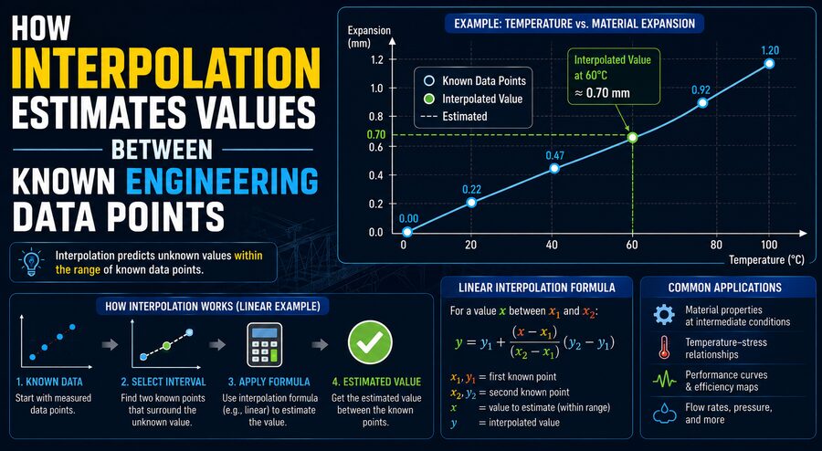
Interpolation is a mathematical technique used to estimate a value between known data points. Instead of performing another experiment or building a completely new model, interpolation uses the relationship between nearby known values to calculate a reasonable estimate.
It is one of the simplest yet most useful numerical methods in engineering.
🔍 What Is Interpolation?
Interpolation estimates an unknown value that lies within the range of known data.
Suppose an experiment provides these measurements:
Temperature = 20°C → Resistance = 110 Ω
Temperature = 30°C → Resistance = 130 Ω
If an engineer wants to estimate resistance at 25°C, the required point lies between the two measurements.
If the relationship is approximately linear, the engineer can interpolate between them.
Because 25°C is exactly halfway between 20°C and 30°C, the estimated resistance is halfway between 110 Ω and 130 Ω:
Resistance at 25°C ≈ 120 Ω
This is the simplest form of interpolation.
The method essentially asks:
“How far is the desired input between the known inputs, and how far should the output move by the same proportion?”
📏 Interpolation vs. Extrapolation
Interpolation should not be confused with extrapolation.
Interpolation estimates values inside the range of known data.
Extrapolation estimates values outside that range.
For example, if measurements are available at 20°C and 30°C:
- Estimating at 25°C = interpolation
- Estimating at 40°C = extrapolation
Interpolation is generally safer because the estimate remains within a region where actual data already exists.
Extrapolation can be much less reliable because the physical relationship may change beyond the measured range.
For this reason, engineers often trust interpolation more readily than extrapolation, provided the underlying data is accurate and sufficiently smooth.
📈 What Is Linear Interpolation?
The most common interpolation technique is linear interpolation.
Linear interpolation assumes that the relationship between two nearby data points can be approximated by a straight line.
Suppose two known points are:
(x₁, y₁) and (x₂, y₂)
The unknown value y at some point x between them can be estimated using:
y = y₁ + [(x − x₁) / (x₂ − x₁)] × (y₂ − y₁)
This formula may look complicated at first, but it simply calculates how far x lies between x₁ and x₂ and applies the same fraction to the change in y.
🧮 A Simple Linear Interpolation Example
Imagine an engineering table showing the viscosity of a fluid:
40°C → 8.0 mPa·s
60°C → 5.0 mPa·s
An engineer needs an approximate viscosity at 50°C.
First, determine where 50°C lies between 40°C and 60°C:
(50 − 40) / (60 − 40) = 10 / 20 = 0.5
So 50°C lies halfway between the two known temperatures.
Next, calculate the change in viscosity:
5.0 − 8.0 = −3.0 mPa·s
Half of that change is:
0.5 × (−3.0) = −1.5
Therefore:
Estimated viscosity = 8.0 − 1.5 = 6.5 mPa·s
So the interpolated viscosity at 50°C is approximately:
6.5 mPa·s
The calculation assumes that viscosity behaves approximately linearly over this relatively small temperature interval.
🧭 Understanding the Interpolation Fraction
The key part of the equation is:
(x − x₁) / (x₂ − x₁)
This quantity tells us where the unknown input lies between the two known values.
Suppose:
x₁ = 100
x₂ = 200
If:
x = 125
then:
(125 − 100) / (200 − 100) = 25 / 100 = 0.25
The desired value lies 25% of the way from the first point to the second.
Therefore, the interpolated output should also move approximately 25% of the way from y₁ toward y₂.
This proportional reasoning is why linear interpolation is intuitive and widely used.
🏗️ Why Engineers Use Interpolation
Engineering data is rarely available at every possible operating condition.
A table containing measurements for every fraction of a degree, every possible pressure, or every machine speed would be enormous and impractical.
Instead, engineers store representative data points and estimate intermediate values when necessary.
Interpolation is commonly used because it is:
- 📊 Simple
- ⚡ Fast
- 🧮 Easy to automate
- 💻 Computationally inexpensive
- 📐 Often sufficiently accurate over small intervals
For many practical engineering calculations, these advantages make interpolation ideal.
🌡️ Interpolation in Thermodynamics
Thermodynamic property tables are a classic example.
Engineers working with steam, refrigerants, gases, and liquids frequently need properties such as:
- Enthalpy
- Entropy
- Specific volume
- Density
- Internal energy
- Saturation pressure
Tables may provide these properties at discrete temperatures or pressures.
Suppose a steam table provides enthalpy at 120°C and 125°C, but the system operates at 123°C.
Interpolation can estimate the enthalpy at the required temperature.
This prevents the engineer from needing an exact experimental measurement for every possible operating condition.
🔩 Material Property Tables
Material properties also vary with temperature and other conditions.
Engineers may interpolate values for:
- Elastic modulus
- Thermal conductivity
- Specific heat
- Yield strength
- Electrical resistivity
- Thermal expansion coefficient
Suppose thermal conductivity is provided at 100°C and 200°C, while a heat-transfer calculation requires the value at 140°C.
Interpolation provides a practical estimate.
However, engineers must verify that the property changes smoothly enough across the interval for the selected interpolation method to be appropriate.
🌊 Fluid Mechanics Applications
Interpolation appears frequently in fluid mechanics.
Engineers may use tables and charts describing:
- Fluid viscosity
- Density
- Drag coefficient
- Friction factor
- Reynolds-number relationships
- Pump performance
For example, a pump manufacturer may provide flow rate and head measurements at selected operating conditions.
If the actual system operates between two test points, interpolation can estimate pump behavior.
Similarly, aerodynamic and hydrodynamic data may require interpolation between measured coefficients.
✈️ Aerospace Engineering
Aircraft and spacecraft engineers rely heavily on numerical datasets.
Wind-tunnel experiments and computational simulations may provide aerodynamic coefficients at selected combinations of:
- Angle of attack
- Mach number
- Reynolds number
- Control-surface position
- Altitude
A flight-control computer may need aerodynamic values at conditions located between measured points.
Interpolation allows it to estimate these values continuously.
For example, lift coefficient might be measured at:
4° angle of attack → CL = 0.40
6° angle of attack → CL = 0.60
At 5°, a simple linear interpolation would estimate:
CL ≈ 0.50
Real aerodynamic databases often require more sophisticated multidimensional interpolation, but the underlying idea remains similar. ✈️
🚗 Automotive Engineering
Vehicle engineers also work with large collections of measured data.
Interpolation can be used in:
- Engine control maps
- Electric motor efficiency maps
- Battery performance tables
- Fuel-injection calibration
- Suspension modeling
- Tire characteristics
An engine-management system, for example, may store values at specific combinations of engine speed and load.
If the engine operates between these points, the controller can interpolate to determine the appropriate fuel quantity or ignition setting.
Modern electronic control units perform calculations like these extremely rapidly.
🔋 Electric Vehicle Battery Models
Battery behavior depends on many variables, including:
- State of charge
- Temperature
- Current
- Cell chemistry
- Battery age
Manufacturers may test battery cells at selected combinations of these variables.
The battery-management system then needs estimates between the measured points.
Interpolation can help estimate quantities such as:
- Open-circuit voltage
- Internal resistance
- Available power
- State-of-charge relationships
Accurate interpolation allows the electronic system to respond smoothly instead of jumping suddenly between discrete table values. ⚡
🗺️ Lookup Tables in Engineering Software
Many engineering systems use lookup tables.
A lookup table stores known input-output relationships.
For example:
| Temperature | Density |
|---|---|
| 20°C | 998 kg/m³ |
| 30°C | 996 kg/m³ |
| 40°C | 992 kg/m³ |
If the software requests density at 35°C, it can locate the surrounding values and interpolate.
Lookup tables are useful because they can represent complex physical behavior without requiring a complicated analytical equation.
This is particularly valuable in embedded systems where computational resources may be limited.
🧮 Bilinear Interpolation
Sometimes a value depends on two independent variables rather than one.
For example, an engine efficiency value might depend on both:
- Engine speed
- Engine torque
In this case, engineers can use bilinear interpolation.
Bilinear interpolation estimates a value within a rectangular grid formed by four surrounding data points.
Instead of interpolating along only one direction, it effectively interpolates across two dimensions.
A common approach is:
- Interpolate between two values along one axis.
- Interpolate between another two values along the same axis.
- Interpolate between those two intermediate results along the second axis.
This technique is widely used in performance maps, simulations, computer graphics, and control systems.
📊 Example of Bilinear Interpolation
Suppose motor efficiency is known at four operating points:
- 2,000 rpm and 100 Nm
- 2,000 rpm and 200 Nm
- 3,000 rpm and 100 Nm
- 3,000 rpm and 200 Nm
If engineers want efficiency at:
2,500 rpm and 150 Nm
the desired operating condition lies between all four known points.
Bilinear interpolation combines those values to estimate efficiency at the center of the grid.
This produces much smoother control behavior than simply selecting whichever stored point happens to be closest.
🧊 Trilinear and Multidimensional Interpolation
Engineering systems can involve more than two variables.
Battery performance, for example, may depend simultaneously on:
- Temperature
- State of charge
- Current
A three-dimensional table may therefore require trilinear interpolation.
Even larger systems may require interpolation across four, five, or more dimensions.
The mathematical concept remains the same: identify surrounding known data and estimate the unknown point based on its relative position within the dataset.
However, computational complexity increases as dimensions are added.
📈 When Linear Interpolation Is Not Enough
Linear interpolation assumes that the relationship between nearby points behaves like a straight line.
That assumption is often reasonable over small intervals.
But some engineering relationships are strongly curved.
Examples may include:
- Chemical reaction rates
- Semiconductor characteristics
- Fluid properties near phase transitions
- Highly nonlinear stress-strain behavior
In such cases, using a straight line may produce noticeable errors.
Engineers can instead use higher-order interpolation methods.
🧮 Polynomial Interpolation
Polynomial interpolation fits a polynomial curve through multiple known points.
Instead of using only two neighboring points, it may use three or more.
A polynomial can capture curvature that a straight line cannot.
Methods include:
- Lagrange interpolation
- Newton polynomial interpolation
For smooth datasets, polynomial interpolation can be highly accurate.
However, using very high-degree polynomials can create unwanted oscillations, particularly near the edges of a dataset.
This behavior is associated with phenomena such as Runge’s phenomenon.
Therefore, simply increasing polynomial order is not always the best strategy.
🌊 Spline Interpolation
A widely used alternative is spline interpolation.
Instead of fitting one large polynomial through the entire dataset, spline interpolation uses smaller polynomial sections.
These sections are joined together smoothly.
One common technique is the cubic spline.
Cubic splines can produce smooth curves while avoiding many of the instability problems associated with high-degree global polynomials.
They are useful when engineers need smooth estimates of:
- Position
- Velocity
- Temperature
- Pressure
- Geometry
- Experimental curves
Computer-aided design and numerical simulation frequently use spline-based techniques.
📐 Interpolation in Structural Engineering
Structural engineers may interpolate between known values when calculating:
- Load factors
- Material properties
- Beam coefficients
- Structural response
- Design-chart values
Many engineering standards contain tables with parameters at selected dimensions or ratios.
If a structure falls between those listed values, interpolation may be permitted or recommended.
However, engineers must always follow the applicable design code because some tables are intentionally conservative and may specify a particular method instead.
🔥 Heat Transfer Applications
Heat-transfer engineers frequently work with temperature-dependent properties.
For example, air’s:
- Density
- Viscosity
- Thermal conductivity
- Specific heat
all change with temperature.
If a calculation requires properties at 375 K while a reference table lists only 350 K and 400 K, interpolation provides a convenient estimate.
This is particularly useful when solving convection and heat-exchanger problems.
⚙️ Manufacturing and Process Control
Factories use sensors that generate data continuously.
Control algorithms may compare real-time measurements against calibration tables.
Interpolation allows machinery to calculate intermediate settings.
Applications can include:
- CNC machine calibration
- Temperature control
- Chemical processing
- Pressure regulation
- Robotic motion
- Flow measurement
By interpolating between calibrated points, systems can respond continuously rather than behaving as though only discrete values exist.
📏 Interpolation in Sensor Calibration
Sensors are not always perfectly linear.
Suppose an industrial pressure sensor produces these calibrated readings:
1.0 V → 20 kPa
2.0 V → 45 kPa
If the sensor outputs 1.4 V, interpolation can estimate the corresponding pressure.
The fractional position is:
(1.4 − 1.0) / (2.0 − 1.0) = 0.4
The pressure difference is:
45 − 20 = 25 kPa
Therefore:
20 + 0.4 × 25 = 30 kPa
The estimated pressure is approximately:
30 kPa
This type of calculation can be performed automatically inside instrumentation electronics.
💻 Interpolation in Engineering Simulations
Numerical simulations divide physical systems into discrete points or elements.
For example, computational fluid dynamics may calculate velocity and pressure at thousands or millions of grid locations.
But an engineer may request the value at a point that does not coincide exactly with a computational node.
Interpolation estimates the value using nearby simulation results.
Similar techniques appear in:
- Finite element analysis
- Computational fluid dynamics
- Weather modeling
- Electromagnetic simulation
- Reservoir modeling
Without interpolation, numerical results would be far less useful between calculated grid points.
🧠 Accuracy Depends on the Data
Interpolation cannot create accuracy that does not exist in the original measurements.
If the known values contain large experimental errors, the interpolated result will also be uncertain.
Its reliability depends on:
- Measurement accuracy
- Distance between known points
- Smoothness of the underlying function
- Chosen interpolation method
- Numerical precision
Closely spaced, high-quality data generally produces better estimates than widely spaced or noisy data.
⚠️ Beware of Sudden Changes
Interpolation works best when the underlying relationship changes smoothly.
Engineers must be cautious near:
- Phase transitions
- Mechanical buckling
- Resonance conditions
- Chemical reaction thresholds
- Electrical switching regions
For example, a fluid property may change dramatically near a boiling or condensation boundary.
A straight-line interpolation across such a transition could be physically misleading.
Understanding the engineering system is therefore just as important as applying the mathematical formula.
🔎 How Engineers Check Interpolation Accuracy
Engineers may validate interpolation by comparing estimates with additional known measurements.
Suppose a dataset includes many experimental points.
An engineer can temporarily remove one point, estimate it using the surrounding values, and compare the interpolated result with the actual measurement.
The difference indicates how well the interpolation method performs.
More advanced systems may calculate statistical errors or uncertainty bounds.
This is especially important when interpolation affects safety-critical calculations.
📉 Interpolation Error
The difference between the estimated interpolated value and the true value is called interpolation error.
For linear interpolation, error tends to increase when:
- Data points are far apart
- The real relationship is strongly curved
- Measurements are noisy
Reducing the distance between known data points often improves accuracy.
Alternatively, engineers may switch to a nonlinear method such as spline interpolation.
🤖 Automated Interpolation in Modern Systems
Today, interpolation is often performed automatically.
Engineering programs such as numerical solvers, simulation packages, spreadsheets, control systems, and embedded software can interpolate thousands or millions of values without requiring manual calculations.
A modern vehicle controller may perform lookup-table interpolation many times per second.
Industrial digital twins may interpolate enormous multidimensional datasets representing machinery behavior.
The calculations are simple individually, but their combined effect is extremely powerful.
🛰️ Interpolation in Navigation and Mapping
Navigation systems also use interpolation.
GPS measurements are obtained at discrete moments, while the system may need to estimate position between updates.
Maps store elevation and terrain values at specific coordinates.
Interpolation can estimate elevation at points located between the stored samples.
Satellite imagery, geographic information systems, and weather maps similarly use interpolation to estimate spatial information.
📊 Choosing the Right Interpolation Method
Engineers select interpolation methods based on the behavior of the data and the required accuracy.
Linear interpolation is excellent when:
- Data points are close together
- Relationships are approximately linear
- Computational simplicity matters
Polynomial interpolation may help when:
- Curvature is significant
- Several reliable data points are available
Spline interpolation is useful when:
- Smoothness is important
- Many data points form a continuous curve
Bilinear or multidimensional interpolation is required when:
- Output depends on multiple input variables
The best method is not necessarily the most mathematically complicated one. A simpler method may be preferable when it provides sufficient accuracy and greater reliability.
🛠️ A Practical Engineering Workflow
A typical engineering interpolation process follows a logical sequence:
- Identify the desired input value.
- Locate the known data points surrounding it.
- Confirm that the target lies inside the data range.
- Examine whether the relationship appears approximately linear.
- Select an appropriate interpolation method.
- Calculate the estimated value.
- Check units and physical reasonableness.
- Consider uncertainty and possible interpolation error.
This final reasonableness check is essential.
If an interpolated result contradicts basic physical expectations, the engineer should investigate rather than blindly accepting the calculation.
🌍 Why Interpolation Is So Important
Engineering constantly converts limited measurements into useful predictions.
It is impossible to experimentally test every possible temperature, pressure, speed, load, voltage, and operating condition.
Interpolation provides a practical bridge between discrete measurements.
It allows engineers to turn tables and datasets into nearly continuous representations of physical behavior.
That capability supports everything from bridges and aircraft to batteries, chemical plants, engines, electronics, and climate models. 🌉✈️🔋
✨ Conclusion
Interpolation estimates values between known engineering data points by determining where an unknown input lies relative to nearby measurements and using that position to estimate the corresponding output.
The simplest form, linear interpolation, assumes that two neighboring data points are connected by a straight line. If the required input lies 30% of the way between two known values, the estimated output is moved approximately 30% between the associated outputs.
More advanced methods such as bilinear interpolation, polynomial interpolation, cubic splines, and multidimensional interpolation extend this idea to nonlinear relationships and complex engineering datasets.
Interpolation is valuable because engineering data is almost always discrete while real operating conditions are continuous. A machine may operate at 1,547 rpm even though measurements exist only at 1,500 and 1,600 rpm. A fluid may be at 73°C while its properties are tabulated at 70°C and 80°C.
Interpolation fills those gaps. 📊
When used carefully, it provides a fast, practical, and mathematically sound way to estimate missing information without repeating expensive experiments or simulations.
Ultimately, interpolation transforms a collection of isolated engineering measurements into a usable picture of what happens between the points—making it one of the most fundamental tools in numerical engineering. 📐⚙️